41.5 Summary statistics

Concise summaries for continuous and categorical variables, plus grouped business KPIs.

skim(tx)

Table 41.2: Data summary

Name	tx
Number of rows	8602
Number of columns	13
_______________________
Column type frequency:
Date	1
factor	3
numeric	9
________________________
Group variables	None

Variable type: Date

skim_variable	n_missing	complete_rate	min	max	median	n_unique
date	0	1	2000-01-01	2015-07-01	2007-10-01	187

Variable type: factor

skim_variable	n_missing	complete_rate	ordered	n_unique	top_counts
city	0	1	FALSE	46	Abi: 187, Ama: 187, Arl: 187, Aus: 187
quarter	0	1	FALSE	4	Q1: 2208, Q2: 2208, Q3: 2116, Q4: 2070
ym	0	1	FALSE	187	200: 46, 200: 46, 200: 46, 200: 46

Variable type: numeric

skim_variable	n_missing	complete_rate	mean	sd	p0	p25	p50	p75	p100	hist
year	0	1.00	2007.30	4.50	2000.00	2003.00	2007.00	2011.00	2.015000e+03	▇▆▆▆▅
month	0	1.00	6.41	3.44	1.00	3.00	6.00	9.00	1.200000e+01	▇▅▅▅▇
sales	568	0.93	549.56	1110.74	6.00	86.00	169.00	467.00	8.945000e+03	▇▁▁▁▁
volume	568	0.93	106858620.78	244933668.97	835000.00	10840000.00	22986824.00	75121388.75	2.568157e+09	▇▁▁▁▁
median	616	0.93	128131.44	37359.58	50000.00	100000.00	123800.00	150000.00	3.042000e+05	▅▇▃▁▁
listings	1424	0.83	3216.90	5968.33	0.00	682.00	1283.00	2953.75	4.310700e+04	▇▁▁▁▁
inventory	1467	0.83	7.17	4.61	0.00	4.90	6.20	8.15	5.590000e+01	▇▁▁▁▁
avg_price	568	0.93	153202.38	48188.98	54782.61	118099.79	142510.87	181806.06	3.626882e+05	▃▇▃▁▁
absorption	1427	0.83	0.18	0.11	0.01	0.12	0.16	0.21	1.650000e+00	▇▁▁▁▁

# City-level yearly KPIs
city_year <- tx %>%
    group_by(city, year) %>%
    summarise(
        n_months      = n(),
        sales_total   = sum(sales, na.rm = TRUE),
        volume_total  = sum(volume, na.rm = TRUE),
        median_price  = median(median, na.rm = TRUE),
        avg_inventory = mean(inventory, na.rm = TRUE),
        .groups = "drop"
    ) %>%
    arrange(city, year)
head(city_year, 10)
#> # A tibble: 10 × 7
#>    city     year n_months sales_total volume_total median_price avg_inventory
#>    <fct>   <int>    <int>       <dbl>        <dbl>        <dbl>         <dbl>
#>  1 Abilene  2000       12        1375    108575000        67100          6.47
#>  2 Abilene  2001       12        1431    114365000        70050          6.62
#>  3 Abilene  2002       12        1516    118675000        67100          5.84
#>  4 Abilene  2003       12        1632    135675000        71850          5.68
#>  5 Abilene  2004       12        1830    159670000        73200          4.56
#>  6 Abilene  2005       12        1977    198855000        92400          3.82
#>  7 Abilene  2006       12        1997    227530000        99900          4.48
#>  8 Abilene  2007       12        2003    232062585       102800          4.96
#>  9 Abilene  2008       12        1651    192520335       106900          6.32
#> 10 Abilene  2009       12        1634    202357756       109050          6.12

# Example visual: price over time for a few major cities
top_cities <- tx %>%
    count(city, sort = TRUE) %>%
    slice_head(n = 6) %>%
    pull(city)

tx %>%
    filter(city %in% top_cities) %>%
    ggplot(aes(date, median, color = city)) +
    geom_line(linewidth = 0.7) +
    scale_y_continuous(labels = scales::dollar_format()) +
    labs(
        title = "Median price over time",
        x = NULL,
        y = "Median price",
        color = "City"
    ) +
    theme_minimal(base_size = 12)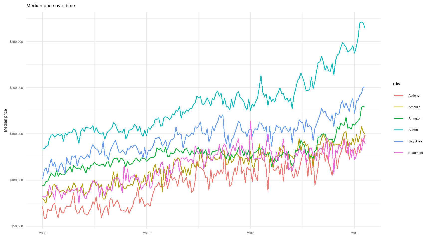

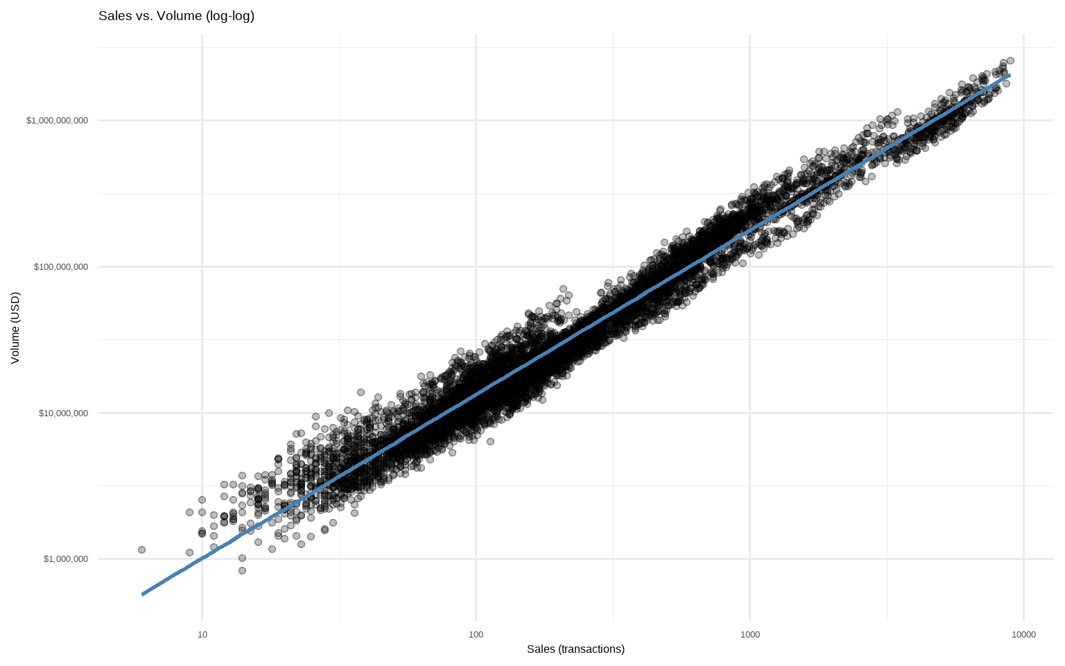
# Volume vs. Sales (log-scale to reduce skew)
tx %>%
    filter(sales > 0, volume > 0) %>%
    ggplot(aes(sales, volume)) +
    geom_point(alpha = 0.25) +
    scale_x_log10() +
    scale_y_log10(labels = scales::dollar_format()) +
    geom_smooth(method = "lm",
                se = FALSE,
                color = "steelblue") +
    labs(title = "Sales vs. Volume (log-log)",
         x = "Sales (transactions)",
         y = "Volume (USD)") +
    theme_minimal(base_size = 12)

---