20 Prediction and Estimation
In modern statistics, econometrics, and machine learning, two primary goals often motivate data analysis:
Prediction: To build a function \(\hat{f}\) that accurately predicts an outcome \(Y\) from observed features (predictors) \(X\).
Estimation or Causal Inference: To uncover and quantify the relationship (often causal) between \(X\) and \(Y\), typically by estimating parameters like \(\beta\) in a model \(Y = g(X; \beta)\).
These goals, while superficially similar, rest on distinct philosophical and mathematical foundations. Below, we explore the difference in detail, illustrating key ideas with formal definitions, theorems, proofs (where relevant), and references to seminal works.
20.1 Conceptual Framing
20.1.1 Predictive Modeling
Predictive modeling focuses on building a function \(\hat{f}: \mathcal{X} \rightarrow \mathcal{Y}\) that maps inputs \(X\) to outputs \(Y\). For simplicity, assume:
- \(X \in \mathbb{R}^p\) (though in practice \(X\) can be images, text, time series, etc.).
- \(Y \in \mathbb{R}\) for regression or \(Y \in \{0, 1\}\) (or other finite set) for classification.
The yardstick for success is the function’s accuracy in out-of-sample predictions, often measured by a loss function \(L(\hat{y}, y)\). We typically choose \(\hat{f}\) to minimize expected loss:
\[ \text{(Predictive Problem)} \quad \hat{f} = \arg \min_{f \in \mathcal{F}} \mathbb{E}[L(f(X), Y)], \]
where \(\mathcal{F}\) is a class of functions (models) and \(\mathbb{E}[\cdot]\) is taken over the joint distribution of \((X, Y)\).
20.1.2 Estimation or Causal Inference
By contrast, estimation or causal inference generally aims to uncover the underlying mechanism: how does \(X\) (or a particular component \(T \subseteq X\)) cause changes in \(Y\)? The canonical problem is to estimate parameters \(\beta\) in a model \(m_\beta(x)\) such that:
\[ Y = m_\beta(X) + \varepsilon, \]
or, in linear form,
\[ Y = X\beta + \varepsilon. \]
A variety of statistical properties—consistency, unbiasedness, efficiency, confidence intervals, hypothesis tests—are relevant here. Causal interpretations usually require assumptions beyond typical i.i.d. sampling: unconfoundedness, exogeneity, or random assignment, so that \(\beta\) indeed captures how changes in \(X\) cause changes in \(Y\).
Key Distinction:
- Prediction does not require that the parameters used in \(\hat{f}\) reflect any real-world mechanism. As long as out-of-sample predictive performance is good, the model is deemed successful—even if it’s a “black box.”
- Causal inference demands interpretability in terms of structural or exogenous relationships. The main objective is consistent estimation of the true (or theoretically defined) parameter \(\beta\), which has an economic, biomedical, or policy interpretation.
20.2 Mathematical Setup
20.2.1 Probability Space and Data
We posit a probability space \((\Omega, \mathcal{F}, P)\) and random variables \((X, Y)\) on it. We typically have an i.i.d. sample \(\{(X_i, Y_i)\}_{i=1}^n\) from the true distribution \(\mathcal{D}\). Let:
\[ (X, Y) \sim \mathcal{D}, \quad (X_i, Y_i) \overset{\text{i.i.d.}}{\sim} \mathcal{D}. \]
In prediction, we train on \(\{(X_i, Y_i)\}_{i=1}^n\) to obtain \(\hat{f}\), and we evaluate on a test point \((\tilde{X}, \tilde{Y})\) drawn from \(\mathcal{D}\). In causal inference, we scrutinize the data generating process carefully, ensuring that we can identify a causal effect. For example, we may require:
- Potential outcomes \(\{Y_i(0), Y_i(1)\}\) for treatment effect settings.
- Unconfoundedness or randomization assumptions.
20.2.2 Loss Functions and Risk
A general framework for both tasks is the risk minimization approach. For a function \(f\), define:
- The population (or expected) risk: \[ \mathcal{R}(f) = \mathbb{E}[L(f(X), Y)]. \]
- The empirical risk (on a sample of size \(n\)): \[ \hat{\mathcal{R}}_n(f) = \frac{1}{n} \sum_{i=1}^n L(f(X_i), Y_i). \]
Prediction: We often solve the empirical risk minimization (ERM) problem:
\[ \hat{f} = \arg \min_{f \in \mathcal{F}} \hat{\mathcal{R}}_n(f), \]
possibly with regularization. The measure of success is \(\mathcal{R}(\hat{f})\), i.e., how well \(\hat{f}\) generalizes beyond the training sample.
Causal/Parameter Estimation: We might define an \(M\)-estimator for \(\beta\) (Newey and McFadden 1994). Consider a function \(\psi(\beta; X, Y)\) such that the true parameter \(\beta_0\) satisfies:
\[ \mathbb{E}[\psi(\beta_0; X, Y)] = 0. \]
The empirical \(M\)-estimator solves
\[ \hat{\beta} = \arg \min_\beta \left\| \frac{1}{n} \sum_{i=1}^n \psi(\beta; X_i, Y_i) \right\|, \]
or equivalently sets it to zero in a method-of-moments sense:
\[ \frac{1}{n} \sum_{i=1}^n \psi(\hat{\beta}; X_i, Y_i) = 0. \]
Properties like consistency (\(\hat{\beta} \overset{p}{\to} \beta_0\)) or asymptotic normality (\(\sqrt{n}(\hat{\beta} - \beta_0) \overset{d}{\to} N(0, \Sigma)\)) are central. The emphasis is on uncovering the true \(\beta_0\) rather than purely predictive accuracy.
20.3 Prediction in Detail
20.3.1 Empirical Risk Minimization and Generalization
In supervised learning, the goal is to find a function \(f\) from a class of candidate models \(\mathcal{F}\) (e.g., linear models, neural networks, tree-based models) that accurately predicts an outcome \(Y\) given an input \(X\). This is typically formulated as an Empirical Risk Minimization problem, where we seek to minimize the average loss over the training data:
\[ \hat{f} = \arg \min_{f \in \mathcal{F}} \frac{1}{n} \sum_{i=1}^n L(f(X_i), Y_i). \]
where \(L(\cdot, \cdot)\) is a loss function that quantifies the error between predictions and actual values. Common choices include:
- Squared Error (Regression): \(L(\hat{y}, y) = (\hat{y} - y)^2\).
- Absolute Error (Regression): \(L(\hat{y}, y) = |\hat{y} - y|\).
- Logistic Loss (Classification): \(L(\hat{p}, y) = -[y \log \hat{p} + (1 - y) \log(1 - \hat{p})]\).
By minimizing empirical risk, we find a function \(\hat{f}\) that best fits the observed data. However, minimizing training error does not guarantee good generalization—the ability of \(\hat{f}\) to perform well on unseen data.
20.3.1.1 Overfitting and Regularization
If \(\mathcal{F}\) is very large or expressive (e.g., deep neural networks with millions of parameters), \(\hat{f}\) can become too complex, learning patterns that exist in the training set but do not generalize to new data. This is called overfitting.
To mitigate overfitting, we introduce regularization, modifying the optimization objective to penalize complex models:
\[ \hat{f}_\lambda = \arg \min_{f \in \mathcal{F}} \left\{ \hat{\mathcal{R}}_n(f) + \lambda \Omega(f) \right\}. \]
where:
\(\hat{\mathcal{R}}_n(f) = \frac{1}{n} \sum_{i=1}^{n} L(f(X_i), Y_i)\) is the empirical risk.
\(\Omega(f)\) is a complexity penalty that discourages overly flexible models.
\(\lambda\) controls the strength of regularization.
Common choices of \(\Omega(f)\) include:
LASSO penalty: \(\|\beta\|_1\) (sparsity constraint in linear models).
Ridge penalty: \(\|\beta\|_2^2\) (shrinking coefficients to reduce variance).
Neural network weight decay: \(\sum w^2\) (prevents exploding weights).
Regularization encourages simpler models, which are more likely to generalize well.
20.3.1.2 Generalization and Statistical Learning Theory
A fundamental question in machine learning is: How well does \(\hat{f}\) perform on unseen data? This is captured by the expected risk:
\[ R(f) = \mathbb{E}[L(f(X), Y)]. \]
Ideally, we want to minimize the gap between the true risk \(R(\hat{f})\) and the best possible risk \(R(f^*)\) within \(\mathcal{F}\):
\[ R(\hat{f}) - \min_{f \in \mathcal{F}} R(f). \]
This difference, called the excess risk, measures how well \(\hat{f}\) generalizes beyond the training sample. Statistical Learning Theory provides theoretical tools to analyze this gap (Vapnik 2013; Hastie, Tibshirani, and Friedman 2009). In particular, it establishes generalization bounds that depend on the capacity of the function class \(\mathcal{F}\).
20.3.1.3 Complexity Measures
Two important ways to quantify the complexity of \(\mathcal{F}\) are
20.3.1.3.1 VC Dimension
The VC dimension measures the ability of a hypothesis class \(\mathcal{F}\) to fit arbitrary labels. Formally, the VC dimension of \(\mathcal{F}\), denoted as \(\operatorname{VC}(\mathcal{F})\), is the largest number of points that can be shattered by some function in \(\mathcal{F}\).
- A set of points is shattered by \(\mathcal{F}\) if, for every possible labeling of these points, there exists a function \(f \in \mathcal{F}\) that perfectly classifies them.
Example 1: Linear Classifiers in 2D
Consider a set of points in \(\mathbb{R}^2\) (the plane).
If \(\mathcal{F}\) consists of linear decision boundaries, we can shatter at most three points in general position (because a single line can separate them in any way).
However, four points cannot always be shattered (e.g., if arranged in an XOR pattern). - Thus, the VC dimension of linear classifiers in \(\mathbb{R}^2\) is 3.
Key Property:
A higher VC dimension means a more expressive model class (higher capacity).
If \(\operatorname{VC}(\mathcal{F})\) is too large, the model can memorize the training set, leading to poor generalization.
20.3.1.3.2 Rademacher Complexity
VC dimension is a combinatorial measure, but Rademacher complexity is a more refined, data-dependent measure of function class flexibility.
Intuition: Rademacher complexity quantifies how well functions in \(\mathcal{F}\) can correlate with random noise. If a function class can fit random labels well, it is too flexible and likely to overfit.
Definition:
Given \(n\) training samples, let \(\sigma_1, \dots, \sigma_n\) be independent Rademacher variables (i.e., random variables taking values \(\pm1\) with equal probability). The empirical Rademacher complexity of \(\mathcal{F}\) is:
\[ \hat{\mathcal{R}}_n(\mathcal{F}) = \mathbb{E}_{\sigma} \left[ \sup_{f \in \mathcal{F}} \frac{1}{n} \sum_{i=1}^{n} \sigma_i f(X_i) \right]. \]
Interpretation:
If \(\hat{\mathcal{R}}_n(\mathcal{F})\) is large, then \(\mathcal{F}\) can fit random noise well \(\Rightarrow\) high risk of overfitting.
If \(\hat{\mathcal{R}}_n(\mathcal{F})\) is small, then \(\mathcal{F}\) is more stable \(\Rightarrow\) better generalization.
Example 2: Linear Models with Bounded Norm
Suppose \(\mathcal{F}\) consists of linear models \(f(X) = w^\top X\), where \(\|w\| \leq C\).
The Rademacher complexity of this class scales as \(\mathcal{O}(C/\sqrt{n})\).
This suggests that controlling the norm of \(w\) (e.g., via Ridge Regression) improves generalization.
20.3.2 Bias-Variance Decomposition
For a regression problem with squared-error loss, a classic decomposition is:
\[ \mathbb{E}_{\text{train}}[(\hat{f}(X) - Y)^2] = \underbrace{(\mathbb{E}[\hat{f}(X)] - f^*(X))^2}_{\text{Bias}^2} + \underbrace{\mathbb{E}[(\hat{f}(X) - \mathbb{E}[\hat{f}(X)])^2]}_{\text{Variance}} + \underbrace{\sigma_\varepsilon^2}_{\text{Irreducible Error}} \]
where \(f^*(X) = \mathbb{E}[Y \mid X]\). Minimizing the sum of bias\(^2\) and variance is key.
In prediction, a small increase in bias is often acceptable if it yields a large reduction in variance—this can improve out-of-sample performance. However, for causal inference, any added bias is problematic if it distorts the interpretation of parameters.
20.3.3 Example: Linear Regression for Prediction
Consider a linear predictor:
\[ \hat{y} = x^\top \hat{\beta}. \]
We choose \(\hat{\beta}\) to minimize:
\[ \sum_{i=1}^n (y_i - x_i^\top \beta)^2 \quad \text{or with a penalty:} \quad \sum_{i=1}^n (y_i - x_i^\top \beta)^2 + \lambda \|\beta\|_2^2. \]
Goal: Achieve minimal prediction error on unseen data \((\tilde{x}, \tilde{y})\).
The estimated \(\hat{\beta}\) might be biased if we use regularization (e.g., ridge). But from a purely predictive lens, that bias can be advantageous if it lowers variance substantially and thus lowers expected prediction error.
20.3.4 Applications in Economics
In economics (and related social sciences), prediction plays an increasingly prominent role (Mullainathan and Spiess 2017; Athey and Imbens 2019):
- Measure Variables: Predicting missing or proxy variables (e.g., predicting income from observable covariates, or predicting individual preferences from online behaviors).
- Embed Prediction Tasks Within Parameter Estimation or Treatment Effects: Sometimes, a first-stage prediction (e.g., imputing missing data or generating prognostic scores) is used as an input for subsequent causal analyses.
- Control for Observed Confounders: Machine learning methods—such as LASSO, random forests, or neural nets—can be used to control for high-dimensional \(X\) when doing partial-out adjustments or residualizing outcomes (Belloni, Chernozhukov, and Hansen 2014; Chernozhukov et al. 2018).
20.4 Parameter Estimation and Causal Inference
20.4.1 Estimation in Parametric Models
In a simple parametric form:
\[ Y = X\beta + \varepsilon, \quad \mathbb{E}[\varepsilon \mid X] = 0, \quad \text{Var}(\varepsilon \mid X) = \sigma^2 I. \]
The Ordinary Least Squares estimator is:
\[ \hat{\beta}_{\text{OLS}} = \arg \min_\beta \|Y - X\beta\|_2^2 = (X^\top X)^{-1} X^\top Y. \]
Under classical assumptions (e.g., no perfect collinearity, homoskedastic errors), \(\hat{\beta}_{\text{OLS}}\) is BLUE—the Best Linear Unbiased Estimator.
In a more general form, parameter estimation, denoted \(\hat{\beta}\), focuses on estimating the relationship between \(y\) and \(x\), often with a view toward causality. In many econometric or statistical settings, we write:
\[ y = x^\top \beta + \varepsilon, \]
or more generally \(y = g\bigl(x;\beta\bigr) + \varepsilon,\) where \(\beta\) encodes the structural or causal parameters we wish to recover.
The core aim is consistency—that is, for large \(n\), we want \(\hat{\beta}\) to converge to the true \(\beta\) that defines the underlying relationship. In other words:
\[ \hat{\beta} \xrightarrow{p} \beta, \quad \text{as } n \to \infty. \]
Some texts phrase it informally as requiring that
\[ \mathbb{E}\bigl[\hat{f}\bigr] = f, \]
meaning the estimator is (asymptotically) unbiased for the true function or parameters.
However, consistency alone may not suffice for scientific inference. One often also examines:
- Asymptotic Normality: \(\sqrt{n}(\hat{\beta} - \beta) \xrightarrow{d} \mathcal{N}(0,\Sigma).\)
- Confidence Intervals: \(\hat{\beta}_j \pm z_{\alpha/2}\,\mathrm{SE}\bigl(\hat{\beta}_j\bigr).\)
- Hypothesis Tests: \(H_0\colon \beta_j = 0 \quad\text{vs.}\quad H_1\colon \beta_j \neq 0.\)
20.4.2 Causal Inference Fundamentals
To interpret \(\beta\) in \(Y = X\beta + \varepsilon\) as “causal,” we typically require that changes in \(X\) (or at least in one component of \(X\)) lead to changes in \(Y\) that are not confounded by omitted variables or simultaneity. In a prototypical potential-outcomes framework (for a binary treatment \(D\)):
- \(Y_i(1)\): outcome if unit \(i\) receives treatment \(D = 1\).
- \(Y_i(0)\): outcome if unit \(i\) receives no treatment \(D = 0\).
The observed outcome \(Y_i\) is
\[ Y_i = D_i Y_i(1) + (1 - D_i) Y_i(0). \]
The Average Treatment Effect (ATE) is:
\[ \tau = \mathbb{E}[Y(1) - Y(0)]. \]
Identification of \(\tau\) requires an assumption like unconfoundedness:
\[ \{Y(0), Y(1)\} \perp D \mid X, \]
i.e., after conditioning on \(X\), the treatment assignment is as-if random. Estimation strategies then revolve around properly adjusting for \(X\).
Such assumptions are not necessary for raw prediction of \(Y\): a black-box function can yield \(\hat{Y} \approx Y\) without ensuring that \(\hat{Y}(1) - \hat{Y}(0)\) is an unbiased estimate of \(\tau\).
20.4.3 Role of Identification
Identification means that the parameter of interest (\(\beta\) or \(\tau\)) is uniquely pinned down by the distribution of observables (under assumptions). If \(\beta\) is not identified (e.g., because of endogeneity or insufficient variation in \(X\)), no matter how large the sample, we cannot estimate \(\beta\) consistently.
In prediction, “identification” is not usually the main concern. The function \(\hat{f}(x)\) could be a complicated ensemble method that just fits well, without guaranteeing any structural or causal interpretation of its parameters.
20.4.4 Challenges
- High-Dimensional Spaces: With large \(p\) (number of predictors), covariance among variables (multicollinearity) can hamper classical estimation. This is the setting of the well-known bias-variance tradeoff (Hastie, Tibshirani, and Friedman 2009; Bishop 2006).
- Endogeneity: If \(x\) is correlated with the error term \(\varepsilon\), ordinary least squares (OLS) is biased. Causal inference demands identifying exogenous variation in \(x\), which requires additional assumptions or designs (e.g., randomization).
- Model Misspecification: If the functional form \(g\bigl(x;\beta\bigr)\) is incorrect, parameter estimates can systematically deviate from capturing the true underlying mechanism.
20.5 Causation versus Prediction
Understanding the relationship between causation and prediction is crucial in statistical modeling. Building on Kleinberg et al. (2015) and Mullainathan and Spiess (2017), consider a scenario where \(Y\) is an outcome variable dependent on \(X\), and we want to manipulate \(X\) to maximize some payoff function \(\pi(X,Y)\). Formally:
\[ \pi(X,Y) = \mathbb{E}\bigl[\,U(X,Y)\bigr] \quad \text{or some other objective measure}. \]
The decision on \(X\) depends on how changes in \(X\) influence \(\pi\). Taking a derivative:
\[ \frac{d\,\pi(X,Y)}{dX} = \frac{\partial \pi}{\partial X}(Y) + \frac{\partial \pi}{\partial Y}\,\frac{\partial Y}{\partial X}. \]
We can interpret the terms:
- \(\displaystyle \frac{\partial \pi}{\partial X}\): The direct dependence of the payoff on \(X\), which can be predicted if we can forecast how \(\pi\) changes with \(X\).
- \(\displaystyle \frac{\partial Y}{\partial X}\): The causal effect of \(X\) on \(Y\), essential for understanding how interventions on \(X\) shift \(Y\).
- \(\displaystyle \frac{\partial \pi}{\partial Y}\): The marginal effect of \(Y\) on the payoff.
Hence, Kleinberg et al. (2015) frames this distinction as one between predicting \(Y\) effectively (for instance, “If I observe \(X\), can I guess \(Y\)?”) versus managing or causing \(Y\) to change via interventions on \(X\). Empirically:
- To predict \(Y\), we model \(\mathbb{E}\bigl[Y\mid X\bigr]\).
- To infer causality, we require identification strategies that isolate exogenous variation in \(X\).
Empirical work in economics, or social science often aims to estimate partial derivatives of structural or reduced-form equations:
- \(\displaystyle \frac{\partial Y}{\partial X}\): The causal derivative; tells us how \(Y\) changes if we intervene on \(X\).
- \(\displaystyle \frac{\partial \pi}{\partial X}\): The effect of \(X\) on payoff, partially mediated by changes in \(Y\).
Without proper identification (e.g., randomization, instrumental variables, difference-in-differences, or other quasi-experimental designs), we risk conflating association (\(\hat{f}\) that predicts \(Y\)) with causation (\(\hat{\beta}\) that truly captures how \(X\) shifts \(Y\)).
To illustrate these concepts, consider the following directed acyclic graph (DAG):
library(ggdag)
library(dagitty)
library(ggplot2)


# Define the DAG structure with custom coordinates
dag <- dagitty('
dag {
  X0 [pos="0,1"]
  X [pos="1,2"]
  Y [pos="1,1"]
  II [pos="1,0"]

  X0 -> Y
  X0 -> II
  X -> Y
  Y -> II
}
')

# Convert to ggdag format with manual layout
dag_plot <- ggdag(dag) +
    theme_void() +
    geom_text(aes(x = 0.5, y = 1.2, label = "Causation"), size = 4) +
    geom_text(aes(x = 0.3, y = 0.5, label = "Prediction"), size = 4)
dag_plot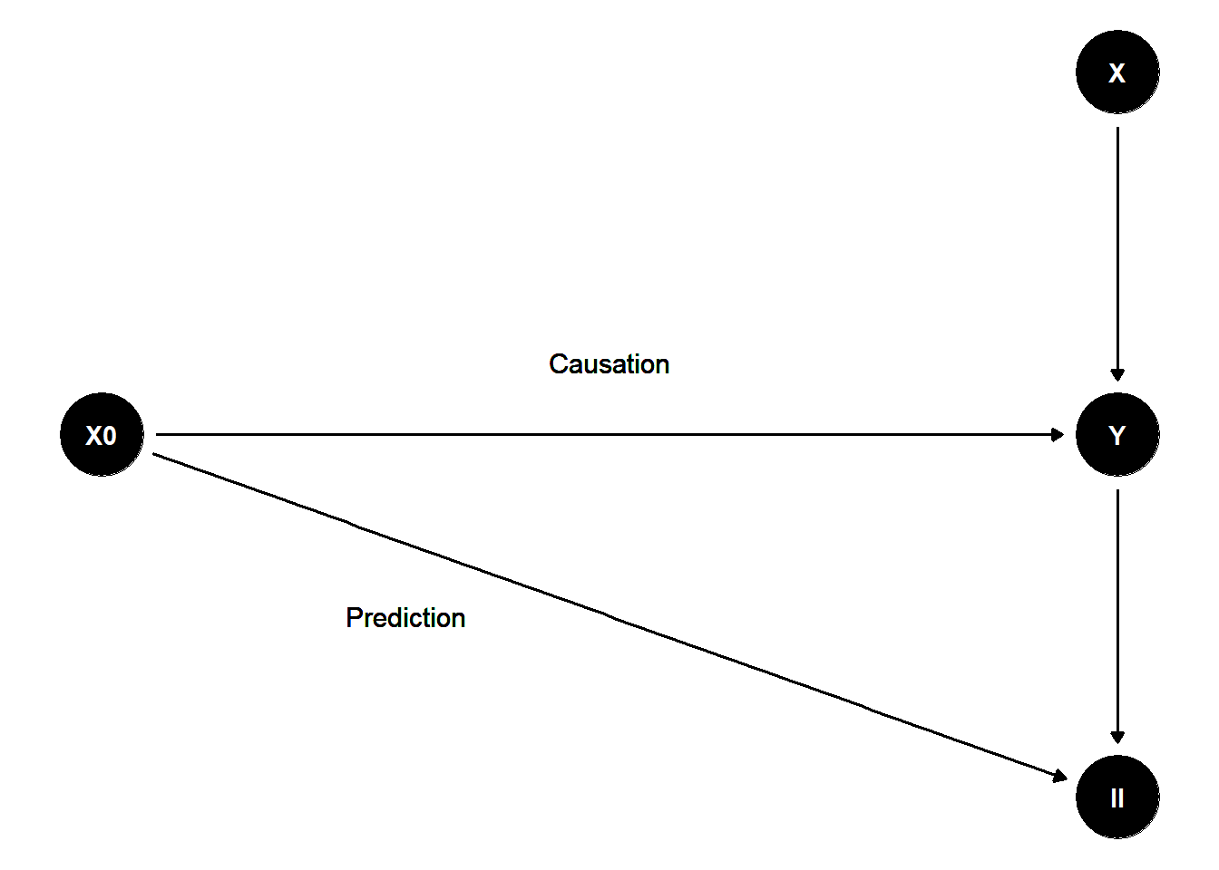
Figure 20.1: Flow Chart
20.6 Illustrative Equations and Mathematical Contrasts
Below, we showcase a few derivations that highlight how predictive modeling vs. causal inference differ in their mathematical structure and interpretation.
20.6.1 Risk Minimization vs. Consistency
Consider a real-valued outcome \(Y\) and predictors \(X\). Let \(\ell(y, \hat{y})\) be a loss function, and define the Bayes regressor \(f^*\) as:
\[ f^* = \arg \min_f \mathbb{E}[\ell(Y, f(X))]. \]
For squared error loss, the Bayes regressor is \(f^*(x) = \mathbb{E}[Y \mid X = x]\).
A learning algorithm tries to approximate \(f^*\). If we parametrize \(f_\beta(x) = x^\top \beta\) and do empirical risk minimization with a large enough sample, \(\beta\) converges to the minimizer of:
\[ \beta^* = \arg \min_\beta \mathbb{E}[(Y - X^\top \beta)^2]. \]
Note that \(\beta^*\) is the solution to \(\mathbb{E}[XX^\top] \beta = \mathbb{E}[XY]\). If \(\text{Cov}(X, X)\) is invertible, then
\[ \beta^* = \text{Cov}(X, X)^{-1} \text{Cov}(X, Y). \]
This \(\beta^*\) is not necessarily the same as the “true” \(\beta_0\) from a structural equation \(Y = X\beta_0 + \varepsilon\) unless \(\mathbb{E}[\varepsilon \mid X] = 0\).
From a predictive standpoint, \(\beta^*\) is the best linear predictor in the sense of mean squared error. From a causal standpoint, we want \(\beta_0\) such that \(\varepsilon\) is mean-independent of \(X\). If that fails, \(\beta^* \neq \beta_0\).
20.6.2 Partial Derivatives vs. Predictions
A powerful way to see the difference is to compare:
- \(\frac{\partial}{\partial x} f^*(x)\) – The partial derivative of the best predictor w.r.t. \(x\). This is about how the model’s prediction changes with \(x\).
- \(\frac{\partial}{\partial x} m_\beta(x)\) – The partial derivative of the structural function \(m_\beta(\cdot)\). This is about how the true outcome \(Y\) changes with \(x\), i.e., a causal effect if \(m_\beta\) is indeed structural.
Unless the model was identified and the assumptions hold (exogeneity, no omitted variables, etc.), the partial derivative from a purely predictive model does not represent the causal effect.
In short: “slopes” from a black-box predictive model are not guaranteed to reflect how interventions on \(X\) would shift \(Y\).
20.6.3 Example: High-Dimensional Regularization
Suppose we have a large number of predictors \(p\), possibly \(p \gg n\). A common approach in both prediction and inference is LASSO:
\[ \hat{\beta}_{\text{LASSO}} = \arg \min_\beta \left\{ \frac{1}{n} \sum_{i=1}^n (y_i - x_i^\top \beta)^2 + \lambda \|\beta\|_1 \right\}. \]
- Prediction: Choose \(\lambda\) to optimize out-of-sample MSE. Some bias is introduced in \(\hat{\beta}\), but the final model might predict extremely well, especially if many true coefficients are near zero.
- Causal Estimation: We must worry about whether the LASSO is shrinking or zeroing out confounders. If a crucial confounder’s coefficient is set to zero, the resulting estimate for a treatment variable’s coefficient will be biased. Therefore, special procedures (like the double/debiased machine learning approach (Chernozhukov et al. 2018)) are introduced to correct for the selection bias or to do post-selection inference (Belloni, Chernozhukov, and Hansen 2014).
The mathematics of “best subset” for prediction vs. valid coverage intervals for parameters diverges significantly.
20.6.4 Potential Outcomes Notation
Let \(D \in \{0, 1\}\) be a treatment indicator, and define potential outcomes:
\[ Y_i(0), Y_i(1). \]
The observed outcome is:
\[ Y_i = D_i Y_i(1) + (1 - D_i) Y_i(0). \]
- Prediction: One might train a model \(\hat{Y} = \hat{f}(X, D)\) to guess \(Y\) from \((X, D)\). That model could be a black box with no guarantee that \(\hat{Y}(1) - \hat{Y}(0)\) is an unbiased estimate of \(Y_i(1) - Y_i(0)\).
- Causal Inference: We want to estimate \(\mathbb{E}[Y(1) - Y(0)]\) or \(\mathbb{E}[Y(1) - Y(0) \mid X = x]\). Identification typically requires \(\{Y(0), Y(1)\} \perp D \mid X\), i.e., after conditioning on \(X\), the treatment assignment is as-if random. Under such an assumption, the difference \(\hat{f}(x, 1) - \hat{f}(x, 0)\) can be interpreted as a causal effect.
20.7 Extended Mathematical Points
We now delve deeper into some mathematical nuances that are especially relevant when distinguishing between predictive vs. causal modeling.
20.7.1 M-Estimation and Asymptotic Theory
\(M\)-Estimators unify many approaches: maximum likelihood, method of moments, generalized method of moments, and quasi-likelihood estimators. Let \(\beta_0\) be the true parameter and define the population criterion function:
\[ Q(\beta) = \mathbb{E}[m(\beta; X, Y)], \]
for some function \(m\). The M-estimator \(\hat{\beta}\) solves:
\[ \hat{\beta} = \arg \max_{\beta \in \Theta} \frac{1}{n} \sum_{i=1}^n m(\beta; X_i, Y_i). \]
(Or \(\arg \min\), depending on convention.)
Under regularity conditions (Newey and McFadden 1994; White 1980), we have:
- Consistency: \(\hat{\beta} \overset{p}{\to} \beta_0\).
- Asymptotic Normality: \(\sqrt{n}(\hat{\beta} - \beta_0) \overset{d}{\to} N(0, \Sigma)\),
where \(\Sigma\) is derived from derivatives of \(m(\cdot; \cdot, \cdot)\) and the distribution of \((X, Y)\).
For prediction, such classical asymptotic properties may be of less interest unless we want to build confidence intervals around predictions. For causal inference, the entire enterprise revolves around these properties to ensure valid inference about \(\beta_0\).
20.7.2 The Danger of Omitted Variables
Consider a structural equation:
\[ Y = \beta_1 X_1 + \beta_2 X_2 + \varepsilon, \quad \mathbb{E}[\varepsilon \mid X_1, X_2] = 0. \]
If we ignore \(X_2\) and regress \(Y\) on \(X_1\) only, the resulting \(\hat{\beta}_1\) can be severely biased:
\[ \hat{\beta}_1 = \arg\min_{b} \sum_{i=1}^n \bigl(y_i - b\,x_{i1}\bigr)^2. \]
The expected value of \(\hat{\beta}_1\) in large samples is:
\[ \beta_1 + \beta_2 \,\frac{\mathrm{Cov}(X_1, X_2)}{\mathrm{Var}(X_1)}. \]
This extra term \(\displaystyle \beta_2 \,\frac{\mathrm{Cov}(X_1, X_2)}{\mathrm{Var}(X_1)}\) is the omitted variables bias. For prediction, omitting \(X_2\) might sometimes be acceptable if \(X_2\) has little incremental predictive value or if we only care about accuracy in some domain. However, for inference on \(\beta_1\), ignoring \(X_2\) invalidates the causal interpretation.
20.7.3 Cross-Validation vs. Statistical Testing
Cross-Validation: Predominantly used in prediction tasks. We split the data into training and validation sets, measure out-of-sample error, and select hyperparameters that minimize CV error.
Statistical Testing: Predominantly used in inference tasks. We compute test statistics (e.g., \(t\)-test, Wald test), form confidence intervals, or test hypotheses about parameters (\(H_0: \beta_j = 0\)).
They serve different objectives:
- CV is about predictive model selection.
- Testing is about scientific or policy conclusions on whether \(\beta_j\) differs from zero (i.e., “Does a particular variable have a causal effect?”).
20.8 Putting It All Together: Comparing Objectives
As an overarching illustration, let \(\hat{f}\) be any trained predictor (ML model, regression, etc.) and let \(\hat{\beta}\) be a parameter estimator from a structural or causal model. Their respective tasks differ:
-
Form of Output
- \(\hat{f}\) is a function from \(\mathcal{X} \to \mathcal{Y}\).
- \(\hat{\beta}\) is a vector of parameters with theoretical meaning.
-
Criterion
- Prediction: Minimizes predictive loss \(\mathbb{E}[L(Y,\hat{f}(X))]\).
- Causal Inference: Seeks \(\beta\) such that \(Y = m_\beta(X)\) is a correct structural representation. Minimizes bias in \(\beta\), or satisfies orthogonality conditions in method-of-moments style, etc.
-
Validity
- Prediction: Usually validated by out-of-sample experiments or cross-validation.
- Estimation: Validated by theoretical identification arguments, assumptions about exogeneity, randomization, or no omitted confounders.
-
Interpretation
- Prediction: “\(\hat{f}(x)\) is our best guess of \(Y\) for new \(x\).”
- Causal Inference: “\(\beta\) measures how \(Y\) changes if we intervene on \(X\).”
20.9 Conclusion
Prediction and Estimation/Causal Inference serve distinctly different roles in data analysis:
Prediction: The emphasis is on predictive accuracy. The final model \(\hat{f}\) may have uninterpretable parameters (e.g., deep neural networks) yet excel at forecasting \(Y\). Bias in parameter estimates is not necessarily problematic if it reduces variance and improves out-of-sample performance.
Estimation/Causal Inference: The emphasis is on obtaining consistent and unbiased estimates of parameters (\(\beta\), or a treatment effect \(\tau\)). We impose stronger assumptions about data collection and the relationship between \(X\) and \(\varepsilon\). The success criterion is whether \(\hat{\beta}\approx\beta_0\) in a formal sense, with valid confidence intervals and robust identification strategies.
Key Takeaway:
If your question is “How do I predict \(Y\) for new \(X\) as accurately as possible?”, you prioritize prediction.
If your question is “How does changing \(X\) (or assigning treatment \(D\)) affect \(Y\) in a causal sense?”, you focus on estimation with a fully developed identification strategy.