36 Endogeneity

In applied research, it’s often tempting to treat regression coefficients as if they represent causal relationships. A positive coefficient on advertising spend, for example, might be interpreted as evidence that increasing ad budgets will increase sales. But such interpretations rely on a critical assumption: that the independent variables we include in a model are exogenous.

This chapter explores the central threat to this assumption: endogeneity.

Endogeneity refers to any situation where an explanatory variable is correlated with the error term in a regression model. When this happens, our coefficient estimates are biased and inconsistent, and any causal claims are invalid.

---

To understand where endogeneity comes from, let’s begin with the familiar linear regression model:

$$\mathbf{Y = X \beta + \epsilon}$$

Where:

• $\mathbf{Y}$ is an $n \times 1$ vector of observed outcomes,
• $\mathbf{X}$ is an $n \times k$ matrix of explanatory variables (including a column of ones for the intercept, if present),
• $\beta$ is a $k \times 1$ vector of unknown parameters,
• $\epsilon$ is an $n \times 1$ vector of unobserved error terms.

The Ordinary Least Squares estimator is:

$$\begin{aligned} \hat{\beta}_{OLS} &= (\mathbf{X}'\mathbf{X})^{-1}(\mathbf{X}'\mathbf{Y}) \\ &= (\mathbf{X}'\mathbf{X})^{-1}(\mathbf{X}'(\mathbf{X\beta + \epsilon})) \\ &= (\mathbf{X}'\mathbf{X})^{-1}(\mathbf{X}'\mathbf{X})\beta + (\mathbf{X}'\mathbf{X})^{-1}(\mathbf{X}'\epsilon) \\ &= \beta + (\mathbf{X}'\mathbf{X})^{-1}(\mathbf{X}'\epsilon) \end{aligned}$$

This derivation makes it clear: OLS is unbiased only if the second term vanishes in expectation. That is:

$$E[(\mathbf{X}'\mathbf{\epsilon})] = 0 \quad \text{or equivalently,} \quad Cov(\mathbf{X}, \epsilon) = 0$$

To produce valid estimates, OLS requires two conditions:

1. Zero Conditional Mean:
   $$E[\epsilon \mid \mathbf{X}] = 0$$ This implies that once we condition on the regressors, there is no systematic error left.

2. No Correlation Between Regressors and Errors:
   $$Cov(\mathbf{X}, \epsilon) = 0$$ This is a stronger requirement. If it fails, we have an endogeneity problem.

The first condition is often satisfied by including an intercept or accounting for the distributional properties of errors. The second condition—lack of correlation between $\mathbf{X}$ and $\epsilon$—is much harder to satisfy, especially in observational data.

Endogeneity violates one of the core assumptions of regression, and it has serious consequences:

• Coefficient bias: Estimates systematically differ from the true parameter values.
• Inconsistency: The bias does not vanish as the sample size increases.
• Incorrect inference: Hypothesis tests and confidence intervals become unreliable.
• Misleading decisions: In business and policy settings, this can lead to costly errors.

---

There are several common sources of endogeneity (Hill et al. 2021). However, most problems fall into two broad categories:

1. Endogenous Treatment

1. Omitted Variable Bias (OVB)

This occurs when a relevant variable is:

• Left out of the model (i.e., omitted),
• Correlated with both the explanatory variable(s) and the outcome.

When is OVB a problem?

• The omitted variable is correlated with an included regressor.
• It also affects the dependent variable.

If either condition fails, there’s no bias.

Example (Economics): We want to estimate the effect of school on earnings, but typical unobservables (e.g., motivation, ability/talent, or self-selection) pose a threat to our identification strategy.

Example (Marketing): Suppose we regress sales on advertising spend, but omit product quality. If higher-quality products get more advertising and also generate more sales, the ad spend coefficient picks up some of the effect of quality—resulting in an upward bias.

Example (Finance): Regressing firm performance on executive compensation might omit executive ability. If more able executives both command higher compensation and deliver better results, OVB leads to biased inferences.

2. Simultaneity (Feedback Effects)

Simultaneity arises when the dependent variable and an explanatory variable are determined jointly, in equilibrium.

Example (Economics): Price and quantity demanded are determined together in supply-and-demand models. A regression of quantity on price without modeling supply will yield a biased estimate of demand sensitivity.

3. Reverse Causality

A special case of simultaneity where the causation runs opposite to what the model assumes.

Example (Health Policy): A naive model might regress health outcomes on insurance coverage. But it’s plausible that people in poor health are more likely to purchase insurance, causing reverse causality.

Over longer time intervals (e.g., yearly business data), reverse causality can look just like simultaneity in terms of its effect on regression estimates.

4. Measurement Errors

Even if a relevant variable is included, imprecise measurement introduces bias.

Classical Measurement Error (in $X$):

• Leads to attenuation bias—estimated coefficients are biased toward zero.
• Occurs frequently in survey data, behavioral measures, and administrative records.

Example (Digital Marketing): Click-through rates or exposure to ads may be tracked with browser cookies or device IDs, but such identifiers are imperfect. The resulting measurement error biases the estimated effect of advertising downward.

---

2. Endogenous Sample Selection

Sample selection becomes a source of endogeneity when inclusion in the sample is related to the outcome variable.

Example (Labor Economics): Estimating the effect of education on wages using only employed individuals excludes those not currently working. If employment is correlated with unobserved traits (e.g., motivation), the wage equation is biased.

---

Summary Table: Types of Endogeneity

Type	Mechanism	Example Context
Omitted Variable Bias	Omitted variable affects both $X$ and $Y$	Managerial talent in finance, brand quality
Simultaneity	$X$ and $Y$ determined jointly	Price $\leftrightarrow$ Demand
Reverse Causality	$Y$ causes $X$ (opposite direction from model assumption)	Health $\to$ Insurance Revenue $\to$ Ad Spend
Measurement Error	$X$ is observed with error	Digital metrics, survey measures
Endogenous Sample Selection	Sample selection is correlated with outcome	Labor force participation, customer panels

---

Endogeneity is not always fatal—if we can identify it and adjust for it, we can still make credible inferences.

1. Control Variables

If you suspect an omitted variable but have data on it, you can include it as a control. This is called a “selection on observables” approach.

However, this strategy is often insufficient because:

• Many important factors are unobserved (e.g., motivation, ability, expectations).
• Measured variables may contain measurement error, creating new biases.

2. Toolbox for Endogeneity

To address more complex cases, including those involving unobservables, we introduce more advanced methods (see Causal Inference Toolbox)

---

36.1 Endogenous Treatment

Endogenous treatment occurs when the variable of interest (the “treatment”) is not randomly assigned and is correlated with unobserved determinants of the outcome. As discussed earlier, this can arise from omitted variables, simultaneity, or reverse causality. But even if the true variable is theoretically exogenous, measurement error can make it endogenous in practice.

This section focuses on how measurement errors, especially in explanatory variables, introduce bias—typically attenuation bias—and why they are a central concern in applied research.

---

36.1.1 Measurement Errors

Measurement error refers to the difference between the true value of a variable and its observed (measured) value.

• Sources of measurement error:
  • Coding errors: Manual or software-induced data entry mistakes.
  • Reporting errors: Self-report bias, recall issues, or strategic misreporting.

Two Broad Types of Measurement Error

1. Random (Stochastic) Error — Classical Measurement Error
   • Noise is unpredictable and averages out in expectation.
   • Error is uncorrelated with the true variable and the regression error.
   • Common in survey data, tracking errors.
2. Systematic (Non-classical) Error — Non-Random Bias
   • Measurement error exhibits consistent patterns across observations.
   • Often arises from:
     • Instrument error: e.g., faulty sensors, uncalibrated scales.
     • Method error: poor sampling, survey design flaws.
     • Human error: judgment errors, social desirability bias.

Key insight:

• Random error adds noise, pushing estimates toward zero.
• Systematic error introduces bias, pushing estimates either upward or downward.

---

36.1.1.1 Classical Measurement Error

36.1.1.1.1 Right-Hand Side Variable

Let’s examine the most common and analytically tractable case: classical measurement error in an explanatory variable.

Suppose the true model is:

$$Y_i = \beta_0 + \beta_1 X_i + u_i$$

But we do not observe $X_i$ directly. Instead, we observe:

$$\tilde{X}_i = X_i + e_i$$

where $e_i$ is the measurement error, assumed classical:

• $E[e_i] = 0$
• $Cov(X_i, e_i) = 0$
• $Cov(e_i, u_i) = 0$

Now, substitute $\tilde{X}_i$ into the regression:

$$\begin{aligned} Y_i &= \beta_0 + \beta_1 ( \tilde{X}_i - e_i ) + u_i \\ &= \beta_0 + \beta_1 \tilde{X}_i + (u_i - \beta_1 e_i) \\ &= \beta_0 + \beta_1 \tilde{X}_i + v_i \end{aligned}$$

where $v_i = u_i - \beta_1 e_i$ is a composite error term.

Since $\tilde{X}_i$ contains $e_i$, and $v_i$ contains $e_i$, we now have:

$$Cov(\tilde{X}_i, v_i) \neq 0$$

This correlation violates the exogeneity assumption and introduces endogeneity.

---

We can derive the asymptotic bias:

$$\begin{aligned} E[\tilde{X}_i v_i] &= E[(X_i + e_i)(u_i - \beta_1 e_i)] \\ &= -\beta_1 Var(e_i) \\ &\neq 0 \end{aligned}$$

This implies:

• If $\beta_1 > 0$, then $\hat{\beta}_1$ is biased downward.
• If $\beta_1 < 0$, then $\hat{\beta}_1$ is biased upward.

This is called attenuation bias: the estimated effect is biased toward zero.

As the variance of the error $Var(e_i)$ increases or $\frac{Var(e_i)}{Var(\tilde{X}_i)} \to 1$, this bias becomes more severe.

---

Attenuation Factor

The OLS estimator based on the noisy regressor is

$$\hat{\beta}_{OLS} = \frac{ \text{cov}(\tilde{X}, Y)}{\text{var}(\tilde{X})} = \frac{\text{cov}(X + e, \beta X + u)}{\text{var}(X + e)}.$$

Using the assumptions of classical measurement error, it follows that:

$$plim\ \hat{\beta}_{OLS} = \beta \cdot \frac{\sigma_X^2}{\sigma_X^2 + \sigma_e^2} = \beta \cdot \lambda,$$

where:

• $\sigma_X^2$ is the variance of the true regressor $X$,
• $\sigma_e^2$ is the variance of the measurement error $e$, and
• $\lambda = \frac{\sigma_X^2}{\sigma_X^2 + \sigma_e^2}$ is called the reliability ratio, signal-to-total variance ratio, or attenuation factor.

Since $\lambda \in (0, 1]$, the bias always attenuates the estimate toward zero. The degree of attenuation bias is:

$$\hat{\beta}_{OLS} - \beta = - (1 - \lambda)\beta,$$

which implies:

• If $\lambda = 1$, then $\hat{\beta}_{OLS} = \beta$ — no bias (no measurement error).
• If $\lambda < 1$, then $\hat{\beta}_{OLS} < \beta$ — attenuation toward zero.

---

Important Notes on Measurement Error

• Data transformations can magnify measurement error.

  Suppose the true model is nonlinear:

  $$y = \beta x + \gamma x^2 + \epsilon,$$

  and $x$ is measured with classical error. Then, the attenuation factor for $\hat{\gamma}$ is approximately the square of the attenuation factor for $\hat{\beta}$:

  $$\lambda_{\hat{\gamma}} \approx \lambda_{\hat{\beta}}^2.$$

  This shows how nonlinear transformations (e.g., squares, logs) can exacerbate measurement error problems.

• Including covariates can increase attenuation bias.

  Adding covariates that are correlated with the mismeasured variable can worsen bias in the coefficient of interest, especially if the measurement error is not accounted for in those covariates.

---

Remedies for Measurement Error

To address attenuation bias caused by classical measurement error, consider the following strategies:

1. Use validation data or survey information to estimate $\sigma_X^2$, $\sigma_e^2$, or $\lambda$ and apply correction methods (e.g., SIMEX, regression calibration).
2. Instrumental Variables Approach
   Use an instrument $Z$ that:
   • Is correlated with the true variable $X$,
   • Is uncorrelated with the regression error $\epsilon$, and
   • Is uncorrelated with the measurement error $e$.
3. Abandon your project
   If no good instruments or validation data exist, and the attenuation bias is too severe, it may be prudent to reconsider the analysis or research question. (Said with love and academic humility.)

---

36.1.1.1.2 Left-Hand Side Variable

Measurement error in the dependent variable (i.e., the response or outcome) is fundamentally different from measurement error in explanatory variables. Its consequences are often less problematic for consistent estimation of regression coefficients (e.g., the zero conditional mean assumption is not violated), but not necessarily for statistical inference (e.g., higher standard errors) or model fit.

---

Suppose we are interested in the standard linear regression model:

$$Y_i = \beta X_i + u_i,$$

but we do not observe $Y_i$ directly. Instead, we observe:

$$\tilde{Y}_i = Y_i + v_i,$$

where:

• $v_i$ is measurement error in the dependent variable,
• $E[v_i] = 0$ (mean-zero),
• $v_i$ is uncorrelated with $X_i$ and $u_i$,
• $v_i$ is homoskedastic and independent across observations.

Be extra careful here!

These are classical‐error assumptions:

1. Mean zero: $\mathbb{E}[v\mid X]=0$.
2. Exogeneity: $v$ is uncorrelated with each regressor and with the structural disturbance $\epsilon$ (i.e., $\operatorname{Cov}(X,v)=\operatorname{Cov}(\epsilon,v)=0$).
3. Homoskedasticity / finite moments for the law‑of‑large‑numbers to apply.

---

The regression we actually estimate is:

$$\tilde{Y}_i = \beta X_i + u_i + v_i.$$

We can define a composite error term:

$$\tilde{u}_i = u_i + v_i,$$

so that the model becomes:

$$\tilde{Y}_i = \beta X_i + \tilde{u}_i.$$

Under the classical-error assumptions, the extra noise simply enlarges the composite error term $\tilde{u}_i$, leaving

$$\hat\beta^{\text{OLS}} =\beta + ( X' X)^{-1} X'(u+v) \;\xrightarrow{p} \beta ,$$

so the estimator remains consistent and only its variance rises.

---

Key Insights

• Unbiasedness and Consistency of $\hat{\beta}$:

  As long as $E[\tilde{u}_i \mid X_i] = 0$, which holds under the classical assumptions (i.e., $E[u_i \mid X_i] = 0$ and $E[v_i \mid X_i] = 0$), the OLS estimator of $\beta$ remains unbiased and consistent.

  This is because measurement error in the left-hand side does not induce endogeneity. The zero conditional mean assumption is preserved.

• Interpretation (Why Econometricians Don’t Panic):

  Econometricians and causal researchers often focus on consistent estimation of causal effects under strict exogeneity. Since $v_i$ just adds noise to the outcome and doesn’t systematically relate to $X_i$, the slope estimate $\hat{\beta}$ remains a valid estimate of the causal effect $\beta$.

• Statistical Implications (Why Statisticians Might Worry):

  Although $\hat{\beta}$ is consistent, the variance of the error term increases due to the added noise $v_i$. Specifically:

  $$\text{Var}(\tilde{u}_i) = \text{Var}(u_i) + \text{Var}(v_i) = \sigma_u^2 + \sigma_v^2.$$

  This leads to:

  • Higher residual variance $\Rightarrow$ lower $R^2$
  • Higher standard errors for coefficient estimates
  • Wider confidence intervals, reducing the precision of inference

  Thus, even though the point estimate is valid, inference becomes weaker: hypothesis tests are less powerful, and conclusions less precise.

---

Practical Illustration

• Suppose $X$ is a marketing investment and $Y$ is sales revenue.
• If sales are measured with noise (e.g., misrecorded sales data, rounding, reporting delays), the coefficient on marketing is still consistently estimated.
• However, uncertainty around the estimate grows: wider confidence intervals might make it harder to detect statistically significant effects, especially in small samples.

---

Summary Table: Measurement Error Consequences

Location of Measurement Error	Bias in $\hat{\beta}$	Consistency	Affects Inference?	Typical Concern
Regressor ($X$)	Yes (attenuation)	No	Yes	Econometric & statistical
Outcome ($Y$)	No	Yes	Yes	Mainly statistical

---

36.1.1.2 Non-Classical Measurement Error

In the classical measurement error model, we assume that the measurement error $\epsilon$ is independent of the true variable $X$ and of the regression disturbance $u$. However, in many realistic data scenarios, this assumption does not hold. Non-classical measurement error refers to cases where:

• $\epsilon$ is correlated with $X$,
• or possibly even correlated with $u$.

Violating the classical assumptions introduces additional and potentially complex biases in OLS estimation.

---

Recall that in the classical measurement error model, we observe:

$$\tilde{X} = X + \epsilon,$$

where:

• $\epsilon$ is independent of $X$ and $u$,
• $E[\epsilon] = 0$.

The true model is:

$$Y = \beta X + u.$$

Then, OLS based on the mismeasured regressor gives:

$$\hat{\beta}_{OLS} = \frac{\text{cov}(\tilde{X}, Y)}{\text{var}(\tilde{X})} = \frac{\text{cov}(X + \epsilon, \beta X + u)}{\text{var}(X + \epsilon)}.$$

With classical assumptions, this simplifies to:

$$plim\ \hat{\beta}_{OLS} = \beta \cdot \frac{\sigma_X^2}{\sigma_X^2 + \sigma_\epsilon^2} = \beta \cdot \lambda,$$

where $\lambda$ is the reliability ratio, which attenuates $\hat{\beta}$ toward zero.

---

Let us now relax the independence assumption and allow for correlation between $X$ and $\epsilon$. In particular, suppose:

• $\text{cov}(X, \epsilon) = \sigma_{X\epsilon} \ne 0$.

Then the probability limit of the OLS estimator becomes:

$$\begin{aligned} plim\ \hat{\beta} &= \frac{\text{cov}(X + \epsilon, \beta X + u)}{\text{var}(X + \epsilon)} \\ &= \frac{\beta (\sigma_X^2 + \sigma_{X\epsilon})}{\sigma_X^2 + \sigma_\epsilon^2 + 2 \sigma_{X\epsilon}}. \end{aligned}$$

We can rewrite this as:

$$\begin{aligned} plim\ \hat{\beta} &= \beta \left(1 - \frac{\sigma_\epsilon^2 + \sigma_{X\epsilon}}{\sigma_X^2 + \sigma_\epsilon^2 + 2 \sigma_{X\epsilon}} \right) \\ &= \beta (1 - b_{\epsilon \tilde{X}}), \end{aligned}$$

where $b_{\epsilon \tilde{X}}$ is the regression coefficient of $\epsilon$ on $\tilde{X}$, or more precisely:

$$b_{\epsilon \tilde{X}} = \frac{\text{cov}(\epsilon, \tilde{X})}{\text{var}(\tilde{X})}.$$

This makes clear that the bias in $\hat{\beta}$ depends on how strongly the measurement error is correlated with the observed regressor $\tilde{X}$. This general formulation nests the classical case as a special case:

• In classical error: $\sigma_{X\epsilon} = 0 \Rightarrow b_{\epsilon \tilde{X}} = \frac{\sigma^2_\epsilon}{\sigma^2_X + \sigma^2_\epsilon} = 1 - \lambda$.

---

Implications of Non-Classical Measurement Error

• When $\sigma_{X\epsilon} > 0$, the attenuation bias can increase or decrease depending on the balance of variances.
• In particular:
  • If more than half of the variance in $\tilde{X}$ is due to measurement error, increasing $\sigma_{X\epsilon}$ increases attenuation.
  • If less than half is due to measurement error, it can actually reduce attenuation.
• This phenomenon is sometimes called mean-reverting measurement error: the measurement error pulls observed values toward the mean, distorting estimates Bound, Brown, and Mathiowetz (2001).

---

36.1.1.2.1 A General Framework for Non-Classical Measurement Error

Bound, Brown, and Mathiowetz (2001) offer a unified matrix framework that accommodates measurement error in both the independent and dependent variables.

Let the true model be:

$$\mathbf{Y = X \beta + \epsilon},$$

but we observe $\tilde{X} = X + U$ and $\tilde{Y} = Y + v$, where:

• $U$ is a matrix of measurement error in $X$,
• $v$ is a vector of measurement error in $Y$.

Then, the observed model becomes:

$$\hat{\beta} = (\tilde{X}' \tilde{X})^{-1} \tilde{X}' \tilde{Y}.$$

Substituting the observed quantities:

$$\begin{aligned} \tilde{Y} &= Y + v = X \beta + \epsilon + v, \\ &= \tilde{X} \beta - U \beta + v + \epsilon. \end{aligned}$$

Hence,

$$\hat{\beta} = (\tilde{X}' \tilde{X})^{-1} \tilde{X}' (\tilde{X} \beta - U \beta + v + \epsilon),$$

which simplifies to:

$$\hat{\beta} = \beta + (\tilde{X}' \tilde{X})^{-1} \tilde{X}' (-U \beta + v + \epsilon).$$

Taking the probability limit:

$$plim\ \hat{\beta} = \beta + plim\ [(\tilde{X}' \tilde{X})^{-1} \tilde{X}' (-U \beta + v)],$$

Now define:

$$W = [U \quad v],$$

and we can express the bias compactly as:

$$plim\ \hat{\beta} = \beta + plim\ [(\tilde{X}' \tilde{X})^{-1} \tilde{X}' W \begin{bmatrix} - \beta \\ 1 \end{bmatrix} ].$$

This formulation highlights a powerful insight:

Bias in $\hat{\beta}$ arises from the linear projection of the measurement errors onto the observed $\tilde{X}$.

This expression does not assert that $v$ necessarily biases $\hat\beta$; it simply makes explicit that bias arises whenever the linear projection of $(U\beta-v)$ onto $\tilde X$ is non‑zero. Three cases illustrate the point:

Case	Key correlation	Consequence for $\hat\beta$
Classical Y‑error only $U\equiv0,\; \operatorname{Cov}(\tilde X,v)=0$	projection term vanishes	Consistent; larger standard errors
Correlated Y‑error $U\equiv0,\; \operatorname{Cov}(\tilde X,v)\neq0$	projection picks up $v$	Biased (attenuation or sign reversal possible)
Both X‑ and Y‑error, independent $\operatorname{Cov}(X,U)\neq0,\; \operatorname{Cov}(\tilde X,v)=0$	$U\beta$ projects onto $\tilde X$	Biased because of $U$, not $v$

Hence, your usual “harmless $Y$-noise” result is the special case in the first row.

---

Practical implications

1. Check assumptions explicitly. If the dataset was generated by self‑reports, simultaneous proxies, or modelled outcomes, it is rarely safe to assume $\operatorname{Cov}(X,v)=0$.

2. Correlated errors in $Y$ can creep in through:

   • Common data‑generating mechanisms (e.g., same survey module records both earnings ($Y$) and hours worked ($X$)).
   • Prediction‑generated variables where $v$ inherits correlation with the features used to build $\tilde Y$.

3. Joint mis‑measurement ($U$ and $v$ correlated) is common in administrative or sensor data; here, even “classical” $v$ with respect to $X$ can correlate with $\tilde X=X+U$.

Measurement error in $Y$ is benign only under strong exogeneity and independence conditions. The Bound–Brown–Mathiowetz matrix form (Bound, Brown, and Mathiowetz 2001) simply shows that once those conditions fail—or once $X$ itself is mis‑measured—the same projection logic that produces attenuation bias for $X$ can also transmit bias from $v$ to $\hat\beta$.

So the rule of thumb you learned is true in its narrow, classical setting, but Bound, Brown, and Mathiowetz (2001) remind us that empirical work often strays outside that safe harbor.

---

Consequences and Correction

• Non-classical error can lead to over- or underestimation, unlike the always-attenuating classical case.
• The direction and magnitude of bias depend on the correlation structure of $X$, $\epsilon$, and $v$.
• This poses serious problems in many survey and administrative data settings where systematic misreporting occurs.

---

Practical Solutions

1. Instrumental Variables
   Use an instrument $Z$ that is correlated with the true variable $X$, but uncorrelated with both measurement error and the regression disturbance. IV can help eliminate both classical and non-classical error-induced biases.

2. Validation Studies
   Use a subset of the data with accurate measures to estimate the structure of measurement error and correct estimates via techniques such as regression calibration, multiple imputation, or SIMEX.

3. Modeling the Error Process
   Explicitly model the measurement error process, especially in longitudinal or panel data (e.g., via state-space models or Bayesian approaches).

4. Binary/Dummy Variable Case
   Non-classical error in binary regressors (e.g., misclassification) also leads to bias, but IV methods still apply. For example, if education level is misreported in survey data, a valid instrument (e.g., policy-based variation) can correct for misclassification bias.

---

Summary

Feature	Classical Error	Non-Classical Error
$\text{Cov}(X, \epsilon)$	0	$\ne 0$
Bias in $\hat{\beta}$	Always attenuation	Can attenuate or inflate
Consistency of OLS	No	No
Effect of Variance Structure	Predictable	Depends on $\sigma_{X\epsilon}$
Fixable with IV	Yes	Yes

In short, non-classical measurement error breaks the comforting regularity of attenuation bias. It can produce arbitrary biases depending on the nature and structure of the error. Instrumental variables and validation studies are often the only reliable tools for addressing this complex problem.

---

36.1.1.3 Solution to Measurement Errors in Correlation Estimation

36.1.1.3.1 Bayesian Correction for Correlation Coefficient

We begin by expressing the Bayesian posterior for a correlation coefficient $\rho$:

$$\begin{aligned} P(\rho \mid \text{data}) &= \frac{P(\text{data} \mid \rho) P(\rho)}{P(\text{data})} \\ \text{Posterior Probability} &\propto \text{Likelihood} \times \text{Prior Probability} \end{aligned}$$

Where:

• $\rho$ is the true population correlation coefficient
• $P(\text{data} \mid \rho)$ is the likelihood function
• $P(\rho)$ is the prior density of $\rho$
• $P(\text{data})$ is the marginal likelihood (a normalizing constant)

With sample correlation coefficient $r$:

$$r = \frac{S_{xy}}{\sqrt{S_{xx} S_{yy}}}$$

According to Schisterman et al. (2003), pp. 3, the posterior density of $\rho$ can be approximated as:

$$P(\rho \mid x, y) \propto P(\rho) \cdot \frac{(1 - \rho^2)^{(n - 1)/2}}{(1 - \rho r)^{n - 3/2}}$$

This approximation leads to a posterior that can be modeled via the Fisher transformation:

• Let $\rho = \tanh(\xi)$, where $\xi \sim N(z, 1/n)$
• $r = \tanh(z)$ is the Fisher-transformed correlation

Using conjugate normal approximations, we derive the posterior for the transformed correlation $\xi$ as:

• Posterior Variance:

$$\sigma^2_{\text{posterior}} = \frac{1}{n_{\text{prior}} + n_{\text{likelihood}}}$$

• Posterior Mean:

$$\mu_{\text{posterior}} = \sigma^2_{\text{posterior}} \left(n_{\text{prior}} \cdot \tanh^{-1}(r_{\text{prior}}) + n_{\text{likelihood}} \cdot \tanh^{-1}(r_{\text{likelihood}})\right)$$

To simplify the mathematics, we may assume a prior of the form:

$$P(\rho) \propto (1 - \rho^2)^c$$

where $c$ controls the strength of the prior. If no prior information is available, we can set $c = 0$ so that $P(\rho) \propto 1$.

---

Example: Combining Estimates from Two Studies

Let:

• Current study: $r_{\text{likelihood}} = 0.5$, $n_{\text{likelihood}} = 200$
• Prior study: $r_{\text{prior}} = 0.2765$, $n_{\text{prior}} = 50205$

Step 1: Posterior Variance

$$\sigma^2_{\text{posterior}} = \frac{1}{50205 + 200} = 0.0000198393$$

Step 2: Posterior Mean

Apply Fisher transformation:

• $\tanh^{-1}(0.2765) \approx 0.2841$
• $\tanh^{-1}(0.5) = 0.5493$

Then:

$$\begin{aligned} \mu_{\text{posterior}} &= 0.0000198393 \times (50205 \times 0.2841 + 200 \times 0.5493) \\ &= 0.0000198393 \times (14260.7 + 109.86) \\ &= 0.0000198393 \times 14370.56 = 0.2850 \end{aligned}$$

Thus, the posterior distribution of $\xi = \tanh^{-1}(\rho)$ is:

$$\xi \sim N(0.2850, 0.0000198393)$$

Transforming back:

• Posterior mean correlation: $\rho = \tanh(0.2850) = 0.2776$
• 95% CI for $\xi$: $0.2850 \pm 1.96 \cdot \sqrt{0.0000198393} = (0.2762, 0.2937)$
• Transforming endpoints: $\tanh(0.2762) = 0.2694$, $\tanh(0.2937) = 0.2855$

The Bayesian posterior distribution for the correlation coefficient is:

• Mean: $\hat{\rho}_{\text{posterior}} = 0.2776$
• 95% CI: $(0.2694,\ 0.2855)$

---

This Bayesian adjustment is especially useful when:

1. There is high sampling variation due to small sample sizes
2. Measurement error attenuates the observed correlation
3. Combining evidence from multiple studies (meta-analytic context)

By leveraging prior information and applying the Fisher transformation, researchers can obtain a more stable and accurate estimate of the true underlying correlation.

# Define inputs
n_new  <- 200
r_new  <- 0.5
alpha  <- 0.05

# Bayesian update function for correlation coefficient
update_correlation <- function(n_new, r_new, alpha) {
  
  # Prior (meta-analysis study)
  n_meta <- 50205
  r_meta <- 0.2765
  
  # Step 1: Posterior variance (in Fisher-z space)
  var_xi <- 1 / (n_new + n_meta)
  
  # Step 2: Posterior mean (in Fisher-z space)
  mu_xi <- var_xi * (n_meta * atanh(r_meta) + n_new * atanh(r_new))
  
  # Step 3: Confidence interval in Fisher-z space
  z_crit    <- qnorm(1 - alpha / 2)
  upper_xi  <- mu_xi + z_crit * sqrt(var_xi)
  lower_xi  <- mu_xi - z_crit * sqrt(var_xi)
  
  # Step 4: Transform back to correlation scale
  mean_rho  <- tanh(mu_xi)
  upper_rho <- tanh(upper_xi)
  lower_rho <- tanh(lower_xi)
  
  # Return all values as a list
  list(
    mu_xi     = mu_xi,
    var_xi    = var_xi,
    upper_xi  = upper_xi,
    lower_xi  = lower_xi,
    mean_rho  = mean_rho,
    upper_rho = upper_rho,
    lower_rho = lower_rho
  )
}


# Run update
updated <-
    update_correlation(n_new = n_new,
                       r_new = r_new,
                       alpha = alpha)

# Display updated posterior mean and confidence interval
cat("Posterior mean of rho:", round(updated$mean_rho, 4), "\n")
#> Posterior mean of rho: 0.2775
cat(
    "95% CI for rho: (",
    round(updated$lower_rho, 4),
    ",",
    round(updated$upper_rho, 4),
    ")\n"
)
#> 95% CI for rho: ( 0.2694 , 0.2855 )

# For comparison: Classical (frequentist) confidence interval around r_new
se_r  <- sqrt(1 / n_new)
z_r   <- qnorm(1 - alpha / 2) * se_r
ci_lo <- r_new - z_r
ci_hi <- r_new + z_r

cat("Frequentist 95% CI for r:",
    round(ci_lo, 4),
    "to",
    round(ci_hi, 4),
    "\n")
#> Frequentist 95% CI for r: 0.3614 to 0.6386

---

36.1.2 Simultaneity

Simultaneity arises when at least one of the explanatory variables in a regression model is jointly determined with the dependent variable, violating a critical assumption for causal inference: temporal precedence.

Why Simultaneity Matters

• In classical regression, we assume that regressors are determined exogenously—they are not influenced by the dependent variable.
• Simultaneity introduces endogeneity, where regressors are correlated with the error term, rendering OLS estimators biased and inconsistent.
• This has major implications in fields like economics, marketing, finance, and social sciences, where feedback mechanisms or equilibrium processes are common.

Real-World Examples

• Demand and supply: Price and quantity are determined together in market equilibrium.
• Sales and advertising: Advertising influences sales, but firms also adjust advertising based on current or anticipated sales.
• Productivity and investment: Higher productivity may attract investment, but investment can improve productivity.

---

36.1.2.1 Simultaneous Equation System

We begin with a basic two-equation structural model:

$$\begin{aligned} Y_i &= \beta_0 + \beta_1 X_i + u_i \quad \text{(Structural equation for } Y) \\ X_i &= \alpha_0 + \alpha_1 Y_i + v_i \quad \text{(Structural equation for } X) \end{aligned}$$

Here:

• $Y_i$ and $X_i$ are endogenous variables — both determined within the system.
• $u_i$ and $v_i$ are structural error terms, assumed to be uncorrelated with the exogenous variables (if any).

The equations form a simultaneous system because each endogenous variable appears on the right-hand side of the other’s equation.

---

To uncover the statistical properties of these equations, we solve for $Y_i$ and $X_i$ as functions of the error terms only:

$$\begin{aligned} Y_i &= \frac{\beta_0 + \beta_1 \alpha_0}{1 - \alpha_1 \beta_1} + \frac{\beta_1 v_i + u_i}{1 - \alpha_1 \beta_1} \\ X_i &= \frac{\alpha_0 + \alpha_1 \beta_0}{1 - \alpha_1 \beta_1} + \frac{v_i + \alpha_1 u_i}{1 - \alpha_1 \beta_1} \end{aligned}$$

These are the reduced-form equations, expressing the endogenous variables as functions of exogenous factors and disturbances.

---

36.1.2.2 Simultaneity Bias in OLS

If we naïvely estimate the first equation using OLS, assuming $X_i$ is exogenous, we get:

$$\text{Bias: } \quad Cov(X_i, u_i) = Cov\left(\frac{v_i + \alpha_1 u_i}{1 - \alpha_1 \beta_1}, u_i\right) = \frac{\alpha_1}{1 - \alpha_1 \beta_1} \cdot Var(u_i)$$

This violates the Gauss-Markov Theorem that regressors be uncorrelated with the error term. The OLS estimator for $\beta_1$ is biased and inconsistent.

---

To allow for identification and estimation, we introduce exogenous variables:

$$\begin{cases} Y_i = \beta_0 + \beta_1 X_i + \beta_2 T_i + u_i \\ X_i = \alpha_0 + \alpha_1 Y_i + \alpha_2 Z_i + v_i \end{cases}$$

Where:

• $X_i$, $Y_i$ — endogenous variables
• $T_i$, $Z_i$ — exogenous variables, not influenced by any variable in the system

---

Solving this system algebraically yields the reduced form model:

$$\begin{cases}\begin{aligned}Y_i &= \frac{\beta_0 + \beta_1 \alpha_0}{1 - \alpha_1 \beta_1} + \frac{\beta_1 \alpha_2}{1 - \alpha_1 \beta_1} Z_i + \frac{\beta_2}{1 - \alpha_1 \beta_1} T_i + \tilde{u}_i \\&= B_0 + B_1 Z_i + B_2 T_i + \tilde{u}_i\end{aligned}\\\begin{aligned}X_i &= \frac{\alpha_0 + \alpha_1 \beta_0}{1 - \alpha_1 \beta_1} + \frac{\alpha_2}{1 - \alpha_1 \beta_1} Z_i + \frac{\alpha_1\beta_2}{1 - \alpha_1 \beta_1} T_i + \tilde{v}_i \\&= A_0 + A_1 Z_i + A_2 T_i + \tilde{v}_i\end{aligned}\end{cases}$$

The reduced form expresses endogenous variables as functions of exogenous instruments, which we can estimate using OLS.

---

Using reduced-form estimates $(A_1, A_2, B_1, B_2)$, we can identify (recover) the structural coefficients:

$$\begin{aligned} \beta_1 &= \frac{B_1}{A_1} \\ \beta_2 &= B_2 \left(1 - \frac{B_1 A_2}{A_1 B_2}\right) \\ \alpha_1 &= \frac{A_2}{B_2} \\ \alpha_2 &= A_1 \left(1 - \frac{B_1 A_2}{A_1 B_2} \right) \end{aligned}$$

---

36.1.2.3 Identification Conditions

Estimation of structural parameters is only possible if the model is identified.

Order Condition (Necessary but Not Sufficient)

A structural equation is identified if:

$$K - k \ge m - 1$$

Where:

• $M$ = total number of endogenous variables in the system

• $m$ = number of endogenous variables in the given equation

• $K$ = number of total exogenous variables in the system

• $k$ = number of exogenous variables appearing in the given equation

• Just-identified: $K - k = m - 1$ (exact identification)

• Over-identified: $K - k > m - 1$ (more instruments than necessary)

• Under-identified: $K - k < m - 1$ (cannot be estimated)

Note: The order condition is necessary but not sufficient. The rank condition must also be satisfied for full identification, which we cover in Instrumental Variables.

This simultaneous equations framework provides the foundation for instrumental variable estimation, where:

• Exogenous variables not appearing in a structural equation serve as instruments.
• These instruments allow consistent estimation of endogenous regressors’ effects.

The reduced-form equations are often used to generate fitted values of endogenous regressors, which are then used in a Two-Stage Least Squares estimation process

---

36.1.3 Reverse Causality

Reverse causality refers to a situation in which the direction of causation is opposite to what is presumed. Specifically, we may model a relationship where variable $X$ is assumed to cause $Y$, but in reality, $Y$ causes $X$, or both influence each other in a feedback loop.

This violates a fundamental assumption for causal inference: temporal precedence — the cause must come before the effect. In the presence of reverse causality, the relationship between $X$ and $Y$ becomes ambiguous, and statistical estimators such as OLS become biased and inconsistent.

---

In a standard linear regression model:

$$Y_i = \beta_0 + \beta_1 X_i + u_i$$

We interpret $\beta_1$ as the causal effect of $X$ on $Y$. However, this interpretation implicitly assumes that:

• $X_i$ is exogenous (uncorrelated with $u_i$)
• Changes in $X_i$ occur prior to or independently of changes in $Y_i$

If $Y_i$ also affects $X_i$, then $X_i$ is not exogenous — it is endogenous, because it is correlated with $u_i$ via the reverse causal path.

---

Reverse causality is especially problematic in observational data where interventions are not randomly assigned. Some key examples include:

• Health and income: Higher income may improve health outcomes, but healthier individuals may also earn more (e.g., due to better productivity or fewer sick days).
• Education and wages: Education raises wages, but higher-income individuals might afford better education — or individuals with higher innate ability (reflected in $u$) pursue more education and also earn more.
• Crime and policing: Increased police presence is often assumed to reduce crime, but high-crime areas are also likely to receive more police resources.
• Advertising and sales: Firms advertise more to boost sales, but high sales may also lead to higher advertising budgets — especially when revenue is reinvested in marketing.

---

To model reverse causality explicitly, consider:

36.1.3.1 System of Equations

$$\begin{aligned} Y_i &= \beta_0 + \beta_1 X_i + u_i \quad &\text{(Y depends on X)} \\ X_i &= \gamma_0 + \gamma_1 Y_i + v_i \quad &\text{(X depends on Y)} \end{aligned}$$

This feedback loop represents a simultaneous system, but where the causality direction is unclear. The two equations indicate that both variables are endogenous.

Even if we estimate only the first equation using OLS, the bias becomes apparent:

$$Cov(X_i, u_i) \ne 0 \quad \Rightarrow \quad \hat{\beta}_1 \text{ is biased}$$

Why? Because $X_i$ is determined by $Y_i$, which itself depends on $u_i$. Thus, $X_i$ indirectly depends on $u_i$.

---

In causal diagram notation (Directed Acyclic Graphs, or DAGs), reverse causality violates the acyclicity assumption. Here’s an example:

• Intended model: $X \rightarrow Y$
• Reality: $X \leftrightarrow Y$ (feedback loop)

This non-directional causality prevents us from interpreting coefficients causally unless additional identification strategies are applied.

---

OLS assumes:

$$E[u_i \mid X_i] = 0$$

Under reverse causality, this condition fails. The resulting estimator $\hat{\beta}_1$ captures both the effect of $X$ on $Y$ and the feedback from $Y$ to $X$, leading to:

• Omitted variable bias: $X_i$ captures unobserved information from $Y_i$
• Simultaneity bias: caused by the endogenous nature of $X_i$

---

36.1.3.2 Distinction from Simultaneity

Reverse causality is a special case of endogeneity, often manifesting as simultaneity. However, the key distinction is:

• Simultaneity: Variables are determined together (e.g., in equilibrium models), and both are modeled explicitly in a system.
• Reverse causality: Only one equation is estimated, and the true causal direction is unknown or opposite to what is modeled.

Reverse causality may or may not involve a full simultaneous system — it’s often unrecognized or assumed away, making it especially dangerous in empirical research.

---

There are no mechanical tests that definitively detect reverse causality, but researchers can:

• Use temporal data (lags): Estimate $Y_{it} = \beta_0 + \beta_1 X_{i,t-1} + u_{it}$ and examine the temporal precedence of variables.
• Apply Granger causality tests in time series (not strictly causal, but helpful diagnostically).
• Use theoretical reasoning to justify directionality.
• Check robustness across different time frames or instrumental variables.

---

36.1.3.3 Solutions to Reverse Causality

The following methods can mitigate reverse causality:

1. Instrumental Variables

• Find a variable $Z$ that affects $X$ but is not affected by $Y$, nor correlated with $u_i$.
• First stage: $X_i = \pi_0 + \pi_1 Z_i + e_i$
• Second stage: $\hat{X}_i$ from the first stage is used in the regression for $Y$.

2. Randomized Controlled Trials (RCTs)

• In experiments, the treatment (e.g., $X$) is assigned randomly and therefore exogenous by design.

3. Natural Experiments / Quasi-Experimental Designs

• Use external shocks or policy changes that affect $X$ but not $Y$ directly (e.g., difference-in-differences, regression discontinuity).

4. Panel Data Methods

• Use fixed-effects or difference estimators to eliminate time-invariant confounders.
• Lag independent variables to examine delayed effects and improve causal direction inference.

5. Structural Equation Modeling

• Estimate a full system of equations to explicitly model feedback.

---

36.1.4 Omitted Variable Bias

Omitted Variable Bias (OVB) arises when a relevant explanatory variable that influences the dependent variable is left out of the regression model, and the omitted variable is correlated with one or more included regressors. This violates the exogeneity assumption of OLS and leads to biased and inconsistent estimators.

Suppose we are interested in estimating the effect of an independent variable $X$ on an outcome $Y$, and the true data-generating process is:

$$Y_i = \beta_0 + \beta_1 X_i + \beta_2 Z_i + u_i$$

However, if we omit $Z_i$ and estimate the model:

$$Y_i = \gamma_0 + \gamma_1 X_i + \varepsilon_i$$

Then the estimate $\hat{\gamma}_1$ may be biased because $X_i$ may be correlated with $Z_i$, and $Z_i$ influences $Y_i$.

---

Let us derive the bias formally.

True model:

$$Y_i = \beta_0 + \beta_1 X_i + \beta_2 Z_i + u_i \quad \text{(1)}$$

Estimated model (with $Z_i$ omitted):

$$Y_i = \gamma_0 + \gamma_1 X_i + \varepsilon_i \quad \text{(2)}$$

Now, substitute the true model into the omitted model:

$$Y_i = \beta_0 + \beta_1 X_i + \beta_2 Z_i + u_i = \gamma_0 + \gamma_1 X_i + \varepsilon_i$$

Comparing both models, the omitted variable becomes part of the new error term:

$$\varepsilon_i = \beta_2 Z_i + u_i$$

Now, consider the OLS assumption:

$$E[\varepsilon_i \mid X_i] = 0 \quad \text{(OLS requirement)}$$

But since $\varepsilon_i = \beta_2 Z_i + u_i$ and $Z_i$ is correlated with $X_i$, we have:

$$Cov(X_i, \varepsilon_i) = \beta_2 Cov(X_i, Z_i) \ne 0$$

Therefore, OLS assumption fails, and $\hat{\gamma}_1$ is biased.

---

Let us calculate the expected value of the OLS estimator $\hat{\gamma}_1$.

From regression theory, when omitting $Z_i$, the expected value of $\hat{\gamma}_1$ is:

$$E[\hat{\gamma}_1] = \beta_1 + \beta_2 \cdot \frac{Cov(X_i, Z_i)}{Var(X_i)}$$

This is the Omitted Variable Bias formula.

Interpretation:
The bias in $\hat{\gamma}_1$ depends on: - $\beta_2$: the true effect of the omitted variable on $Y$ - $Cov(X_i, Z_i)$: the correlation between $X$ and the omitted variable $Z$

---

36.1.4.1 Direction of the Bias

• If $\beta_2 > 0$ and $Cov(X_i, Z_i) > 0$: $\hat{\gamma}_1$ is upward biased
• If $\beta_2 < 0$ and $Cov(X_i, Z_i) > 0$: $\hat{\gamma}_1$ is downward biased
• If $Cov(X_i, Z_i) = 0$: No bias, even if $Z_i$ is omitted

Note: Uncorrelated omitted variables do not bias the OLS estimator, although they may reduce precision.

---

36.1.4.2 Practical Example: Education and Earnings

Suppose we model:

$$\text{Earnings}_i = \gamma_0 + \gamma_1 \cdot \text{Education}_i + \varepsilon_i$$

But the true model includes ability ($Z_i$):

$$\text{Earnings}_i = \beta_0 + \beta_1 \cdot \text{Education}_i + \beta_2 \cdot \text{Ability}_i + u_i$$

Omitting “ability” — a determinant of both education and earnings — leads to bias in the estimated effect of education:

• If more able individuals pursue more education and ability raises earnings ($\beta_2 > 0$), then $\hat{\gamma}_1$ overstates the true return to education.

---

36.1.4.3 Generalization to Multiple Regression

In models with multiple regressors, omitting a relevant variable that is correlated with at least one included regressor will bias all coefficients affected by the correlation structure.

For example:

$$Y_i = \beta_0 + \beta_1 X_{1i} + \beta_2 X_{2i} + u_i$$

If $X_2$ is omitted, and $Cov(X_1, X_2) \ne 0$, then:

$$E[\hat{\gamma}_1] = \beta_1 + \beta_2 \cdot \frac{Cov(X_1, X_2)}{Var(X_1)}$$

---

36.1.4.4 Remedies for OVB

1. Include the omitted variable

• If $Z$ is observed, include it in the regression model.

2. Use Instrumental Variables

• If $Z$ is unobserved but $X$ is endogenous, find an instrument $W$:

  • Relevance: $Cov(W, X) \ne 0$
  • Exogeneity: $Cov(W, u) = 0$

3. Use Panel Data Methods

• Fixed Effects: eliminate time-invariant omitted variables.
• Difference-in-Differences: exploit temporal variation to isolate effects.

4. Experimental Designs

• Randomization ensures omitted variables are orthogonal to treatment, avoiding bias.

---

36.2 Endogenous Sample Selection

Endogenous sample selection arises in observational or non-experimental research whenever the inclusion of observations (or assignment to treatment) is not random, and the same unobservable factors influencing selection also affect the outcome of interest. This scenario leads to biased and inconsistent estimates of causal parameters (e.g., Average Treatment Effect) if not properly addressed.

This problem was first formalized in the econometric literature by J. Heckman (1974), J. J. Heckman (1976b), and J. J. Heckman (1979), whose work addressed the issue in the context of labor force participation among women. Later, Amemiya (1984) generalize the method. Now, it has since been applied widely across social sciences, epidemiology, marketing, and finance.

Endogenous sample selection is often conflated with general selection bias, but it is important to understand that sample selection refers specifically to the inclusion of observations into the estimation sample, not just to assignment into treatment (i.e., selection bias).

This problem comes in many names such as self-selection problem, incidental truncation, or omitted variable (i.e., the omitted variable is how people were selected into the sample). Some disciplines consider nonresponse/selection bias as sample selection:

• When unobservable factors that affect who is in the sample are independent of unobservable factors that affect the outcome, the sample selection is not endogenous. Hence, the sample selection is ignorable and estimator that ignores sample selection is still consistent.
• When the unobservable factors that affect who is included in the sample are correlated with the unobservable factors that affect the outcome, the sample selection is endogenous and not ignorable, because estimators that ignore endogenous sample selection are not consistent (we don’t know which part of the observable outcome is related to the causal relationship and which part is due to different people were selected for the treatment and control groups).

Many evaluation studies use observational data, and in such data:

• Participants are not randomly assigned.
• Treatment or exposure is determined by individual or institutional choices.
• Counterfactual outcomes are not observed.
• The treatment indicator is often endogenous.

Some notable terminologies include:

1. Truncation: Occurs when data are collected only from a restricted subpopulation based on the value of a variable.
   • Left truncation: Values below a threshold are excluded (e.g., only high-income individuals are surveyed).
   • Right truncation: Values above a threshold are excluded.
2. Censoring: Occurs when the variable is observed but coarsened beyond a threshold.
   • E.g., incomes below a certain level are coded as zero; arrest counts above a threshold are top-coded.
3. Incidental Truncation: Refers to selection based on a latent variable (e.g., employment decisions), not directly observed. This is what makes Heckman’s model distinct.
   • Also called non-random sample selection.
   • The error in the outcome equation is correlated with the selection indicator.

Researchers often categorize self-selection into:

• Negative (Mitigation-Based) Selection: Individuals select into a treatment or sample to address an existing problem, so they start off with worse potential outcomes.
  • Bias direction: Underestimates true treatment effects (makes the treatment look less effective than it is).
  • Individuals select into treatment to combat a problem they already face.
  • Examples:
    • People at high risk of severe illness (e.g., elderly or immunocompromised individuals) are more likely to get vaccinated. If we compare vaccinated vs. unvaccinated individuals without adjusting for risk factors, we might mistakenly conclude that vaccines are ineffective simply because vaccinated individuals had worse initial health conditions.
    • Evaluating the effect of job training programs—unemployed individuals with the greatest difficulty finding jobs are most likely to enroll, leading to underestimated program benefits.
• Positive (Preference-Based) Selection: Individuals select into a treatment or sample because they have advantageous traits, preferences, or resources. Hence, those who take treatment are systematically better off compared to those who do not.
  • Bias direction: Overestimates true treatment effects (makes the treatment look more effective than it is).
  • Individuals select into treatment because they inherently prefer it, rather than because of an underlying problem.
  • Examples:
    • People who are health-conscious and physically active are more likely to join a fitness program. If we compare fitness program participants to non-participants, we might falsely attribute their better health outcomes to the program, when in reality, their pre-existing lifestyle contributed to their improved health.
    • Evaluating the effect of private school education—students who attend private schools often come from wealthier families with greater academic support, making it difficult to isolate the true impact of the school itself.

Both forms of selection reflect correlation between unobservables (driving selection) and potential outcomes—the hallmark of endogenous selection bias.

---

Some seminal applied works in this area include:

1. Labor Force Participation (J. Heckman 1974)

• Wages are observed only for women who choose to work.
• Unobservable preferences (reservation wages) drive participation.
• Ignoring this leads to biased estimates of the returns to education.

2. Union Membership (Lewis 1986)

• Wages differ between union and non-union workers.
• But union membership is not exogenous—workers choose to join based on anticipated benefits.
• Naïve OLS yields biased estimates of union premium.

3. College Attendance (Card 1999, 2001)

• Comparing income of college graduates vs. non-graduates.
• Attending college is a choice based on expected gains, ability, or family background.
• A treatment effect model (described next) is more appropriate here.

---

36.2.1 Unifying Model Frameworks

Though often conflated, there are several overlapping models to address endogenous selection:

1. Sample Selection Model (J. J. Heckman 1979): Outcome is unobserved if an agent is not selected into the sample.
2. Treatment Effect Model: Outcome is observed for both groups (treated vs. untreated), but treatment assignment is endogenous.
3. Heckman-Type / Control Function Approaches: Decompose the endogenous regressor or incorporate a correction term (Inverse Mills Ratio or residual) to control for endogeneity.

All revolve around the challenge: unobserved factors affect both who is included (or treated) and outcomes.

To formalize the problem, we consider the outcome and selection equations. Let:

• $y_i$: observed outcome (e.g., wage)
• $x_i$: covariates affecting outcome
• $z_i$: covariates affecting selection
• $w_i$: binary indicator for selection into the sample (e.g., employment)

36.2.1.1 Sample Selection Model

We begin with an outcome equation, which describes the variable of interest $y_i$. However, we only observe $y_i$ if a certain selection mechanism indicates it is part of the sample. That mechanism is captured by a binary indicator $w_i = 1$. Formally, the observed outcome equation is:

$$\begin{aligned} y_i &= x_i' \beta + \varepsilon_i, \quad &\text{(Observed only if } w_i = 1\text{)}, \\ \varepsilon_i &\sim N(0, \sigma_\varepsilon^2). \end{aligned}$$

Here, $x_i$ is a vector of explanatory variables (or covariates) that explain $y_i$. The noise term $\varepsilon_i$ is assumed to be normally distributed with mean zero and variance $\sigma_\varepsilon^2$. However, because we only see $y_i$ for those cases in which $w_i = 1$, we must account for how the selection occurs.

Next, we specify the selection equation via a latent index model. Let $w_i^*$ be an unobserved latent variable:

$$\begin{aligned} w_i^* &= z_i' \gamma + u_i, \\ w_i &= \begin{cases} 1 & \text{if } w_i^* > 0, \\ 0 & \text{otherwise}. \end{cases} \end{aligned}$$

Here, $z_i$ is a vector of variables that influence whether or not $y_i$ is observed. In practice, $z_i$ may overlap with $x_i$, but can also include variables not in the outcome equation. For identification, we normalize $\mathrm{Var}(u_i) = 1$. This is analogous to the probit model’s standard normalization.

Because $w_i = 1$ exactly when $w_i^* > 0$, this event occurs if $u_i \ge -\,z_i' \gamma$. Therefore,

$$\begin{aligned} P(w_i = 1) &= P\bigl(u_i \ge -z_i' \gamma\bigr),\\ &= 1 - \Phi\bigl(-z_i'\gamma\bigr), \\ &= \Phi\bigl(z_i'\gamma\bigr), \end{aligned}$$

where we use the symmetry of the standard normal distribution.

We assume $(\varepsilon_i, u_i)$ are jointly normally distributed with correlation $\rho$. In other words,

$$\begin{pmatrix} \varepsilon_i \\ u_i \end{pmatrix} \;\sim\; \mathcal{N} \!\Biggl( \begin{pmatrix} 0 \\ 0 \end{pmatrix}, \begin{pmatrix} \sigma^2_\varepsilon & \rho \,\sigma_\varepsilon \\ \rho \,\sigma_\varepsilon & 1 \end{pmatrix} \Biggr).$$

• If $\rho = 0$, the selection is exogenous: whether $y_i$ is observed is unrelated to unobserved determinants of $y_i$.
• If $\rho \neq 0$, sample selection is endogenous. Failing to model this selection mechanism leads to biased estimates of $\beta$.

Interpreting $\rho$

• $\rho > 0$: Individuals with higher unobserved components in $\varepsilon_i$ (and thus typically larger $y_i$) are more likely to appear in the sample. (Positive selection)
• $\rho < 0$: Individuals with higher unobserved components in $\varepsilon_i$ are less likely to appear. (Negative selection)
• $\rho = 0$: No endogenous selection. Observed outcomes are effectively random with respect to the unobserved part of $y_i$.

In empirical practice, $\rho$ signals the direction of bias one might expect if the selection process is ignored.

Often, it is helpful to visualize how part of the distribution of $u_i$ (the error in the selection equation) is truncated based on the threshold $w_i^*>0$. Below is a notional R code snippet that draws a normal density and shades the region where $u_i > -z_i'\gamma$.

x = seq(-3, 3, length = 200)
y = dnorm(x, mean = 0, sd = 1)
plot(x,
     y,
     type = "l",
     main =  bquote("Probabibility distribution of" ~ u[i]))

x_shaded = seq(0.3, 3, length = 100)
y_shaded = dnorm(x_shaded, 0, 1)
polygon(c(0.3, x_shaded, 3), c(0, y_shaded, 0), col = "gray")

text(1, 0.1, expression(1 - Phi(-z[i] * gamma)))
arrows(-0.5, 0.1, 0.3, 0, length = 0.15)
text(-0.5, 0.12, expression(-z[i] * gamma))
legend("topright",
       "Gray = Prob of Observed",
       pch = 1,
       inset = 0.02)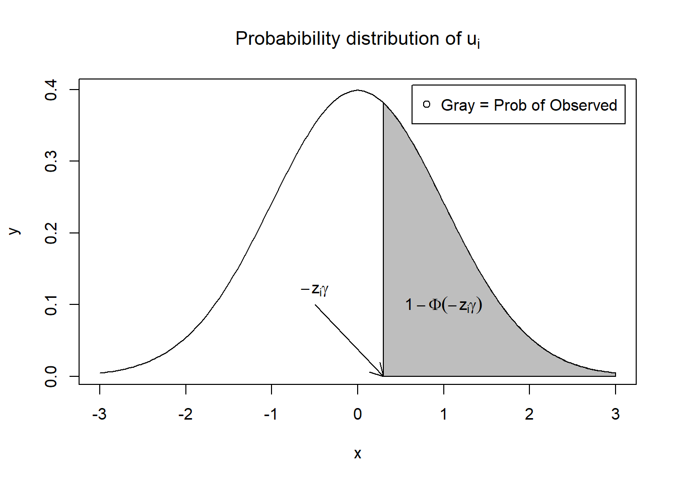

In this figure, the gray‐shaded area represents $u_i > -z_i'\gamma$. Observations in that range are included in the sample. If $\rho\neq 0$, then the unobserved factors that drive $u_i$ also affect $\varepsilon_i$, causing a non‐representative sample of $\varepsilon_i$.

A core insight of the Heckman model is the conditional expectation of $y_i$ given $w_i=1$:

$$E\bigl(y_i \mid w_i = 1\bigr) \;=\; E\bigl(y_i \mid w_i^*>0\bigr) \;=\; E\bigl(x_i'\beta + \varepsilon_i \mid u_i > -z_i'\gamma\bigr).$$

Since $x_i'\beta$ is nonrandom (conditional on $x_i$), we get

$$E\bigl(y_i \mid w_i=1\bigr) = x_i'\beta + E\bigl(\varepsilon_i \mid u_i > -z_i'\gamma\bigr).$$

From bivariate normal properties:

$$\varepsilon_i \,\bigl\lvert\, u_i=a \;\sim\; N\!\Bigl(\rho\,\sigma_{\varepsilon}\cdot a,\; (1-\rho^2)\,\sigma_{\varepsilon}^2\Bigr).$$

Thus,

$$E\bigl(\varepsilon_i \mid u_i > -z_i'\gamma\bigr) =\; \rho\,\sigma_{\varepsilon}\, E\bigl(u_i \mid u_i > -z_i'\gamma\bigr).$$

If $U\sim N(0,1)$, then

$$E(U \mid U>a) = \frac{\phi(a)}{1-\Phi(a)} = \frac{\phi(a)}{\Phi(-a)},$$ where $\phi$ is the standard normal pdf, $\Phi$ is the cdf. By symmetry, $\phi(-a)=\phi(a)$ and $\Phi(-a)=1-\Phi(a)$. Letting $a = -\,z_i'\gamma$ yields

$$E\bigl(U \mid U > -z_i'\gamma\bigr) = \frac{\phi(-z_i'\gamma)}{1-\Phi(-z_i'\gamma)} = \frac{\phi(z_i'\gamma)}{\Phi(z_i'\gamma)}.$$

Define the Inverse Mills Ratio (IMR) as

$$\lambda(x) = \frac{\phi(x)}{\Phi(x)}.$$

Hence,

$$E\bigl(\varepsilon_i \mid u_i > -z_i'\gamma\bigr) = \rho\,\sigma_{\varepsilon}\,\lambda\bigl(z_i'\gamma\bigr),$$ and therefore

$$\boxed{ E\bigl(y_i \mid w_i=1\bigr) = x_i'\beta \;+\; \rho\,\sigma_{\varepsilon}\, \frac{\phi\bigl(z_i'\gamma\bigr)}{\Phi\bigl(z_i'\gamma\bigr)}. }$$

This extra term is the so‐called Heckman correction.

The IMR appears in the two‐step procedure as a regressor for bias correction. It has useful derivatives:

$$\frac{d}{dx}\Bigl[\text{IMR}(x)\Bigr] = \frac{d}{dx}\Bigl[\frac{\phi(x)}{\Phi(x)}\Bigr] = -x\,\text{IMR}(x)\;-\;\bigl[\text{IMR}(x)\bigr]^2.$$

This arises from the quotient rule and the fact that $\phi'(x)=-x\phi(x)$, $\Phi'(x)=\phi(x)$. The derivative property also helps in interpreting marginal effects in selection models.

---

36.2.1.2 Treatment Effect (Switching) Model

While the sample selection model is used when outcome is only observed for one group (e.g., $D = 1$), the treatment effect model is used when outcomes are observed for both groups, but treatment assignment is endogenous.

Treatment Effect Model Equations:

• Outcome: $$y_i = x_i' \beta + D_i \delta + \varepsilon_i$$
• Selection: $$D_i^* = z_i' \gamma + u_i \\ D_i = 1 \text{ if } D_i^* > 0$$

Where:

• $D_i$ is the treatment indicator.

• $(\varepsilon_i, u_i)$ are again bivariate normal with correlation $\rho$.

The treatment effect model is sometimes called a switching regression.

36.2.1.3 Heckman-Type vs. Control Function

• Heckman Sample Selection: Insert an Inverse Mills Ratio (IMR) to adjust the outcome equation for non-random truncation.
• Control Function: Residual-based or predicted-endogenous-variable approach that mirrors IV logic, but typically still requires an instrument or parametric assumption.

Differences between Heckman Sample Selection vs. Heckman-type correction

	Heckman Sample Selection Model	Heckman-Type Corrections
When	Only observes one sample (treated), addressing selection bias directly.	Two samples are observed (treated and untreated), known as the control function approach.
Model	Probit	OLS (even for dummy endogenous variable)
Integration of 1st stage	Also include a term (called Inverse Mills ratio) besides the endogenous variable.	Decompose the endogenous variable to get the part that is uncorrelated with the error terms of the outcome equation. Either use the predicted endogenous variable directly or include the residual from the first-stage equation.
Advantages and Assumptions	Provides a direct test for endogeneity via the coefficient of the inverse Mills ratio but requires the assumption of joint normality of errors.	Does not require the assumption of joint normality, but can’t test for endogeneity directly.

---

36.2.2 Estimation Methods

36.2.2.1 Heckman’s Two-Step Estimator (Heckit)

Step 1: Estimate Selection Equation with Probit

We estimate the probability of being included in the sample: $$P(w_i = 1 \mid z_i) = \Phi(z_i' \gamma)$$

From the estimated model, we compute the Inverse Mills Ratio (IMR): $$\lambda_i = \frac{\phi(z_i' \hat{\gamma})}{\Phi(z_i' \hat{\gamma})}$$

This term captures the expected value of the error in the outcome equation, conditional on selection.

Step 2: Include IMR in Outcome Equation

We then estimate the regression: $$y_i = x_i' \beta + \delta \lambda_i + \nu_i$$

• If $\delta$ is significantly different from 0, selection bias is present.
• $\lambda_i$ corrects for the non-random selection.
• OLS on this augmented model yields consistent estimates of $\beta$ under the joint normality assumption.
• Pros: Conceptually simple; widely used.
• Cons: Relies heavily on the bivariate normal assumption for $(\varepsilon_i, u_i)$. If no good exclusion variable is available, identification rests on the functional form.

Specifically, the model can be identified without an exclusion restriction, but in such cases, identification is driven purely by the non-linearity of the probit function and the normality assumption (through the IMR). This is fragile.

• With strong exclusion restriction for the covariate in the correction equation, the variation in this variable can help identify the control for selection.
• With weak exclusion restriction, and the variable exists in both steps, it’s the assumed error structure that identifies the control for selection (J. Heckman and Navarro-Lozano 2004).
• In management, Wolfolds and Siegel (2019) found that papers should have valid exclusion conditions, because without these, simulations show that results using the Heckman method are less reliable than those obtained with OLS.

For robust identification, we prefer an exclusion restriction:

• A variable that affects selection (through $z_i$) but not the outcome.
• Example: Distance to a training center might affect the probability of enrollment, but not post-training income.

Without such a variable, the model relies solely on functional form.

The Heckman two-step estimation procedure is less efficient than FIML. One key limitation is that the two-step estimator does not fully exploit the joint distribution of the error terms across equations, leading to a loss of efficiency. Moreover, the two-step approach may introduce measurement error in the second stage. This arises because the inverse Mills ratio used in the second stage is itself an estimated regressor, which can lead to biased standard errors and inference.

###########################
#   SIM 1: Heckman 2-step #
###########################
suppressPackageStartupMessages(library(MASS))

set.seed(123)
n <- 1000
rho <- 0.5
beta_true <- 2

gamma_true <- 1.0
Sigma <- matrix(c(1, rho, rho, 1), 2)
errors <- mvrnorm(n, c(0,0), Sigma)

epsilon <- errors[,1]
u       <- errors[,2]

x <- rnorm(n)
w <- rnorm(n)

# Selection
z_star <- w*gamma_true + u
z <- ifelse(z_star>0,1,0)

# Outcome

y_star <- x * beta_true + epsilon
# Observed only if z=1
y_obs <- ifelse(z == 1, y_star, NA)

# Step 1: Probit
sel_mod <- glm(z ~ w, family = binomial(link = "probit"))
z_hat <- predict(sel_mod, type = "link")
lambda_vals <- dnorm(z_hat) / pnorm(z_hat)

# Step 2: OLS on observed + IMR
data_heck <- data.frame(y = y_obs,
                        x = x,
                        imr = lambda_vals,
                        z = z)
observed_data <- subset(data_heck, z == 1)
heck_lm <- lm(y ~ x + imr, data = observed_data)
summary(heck_lm)
#> 
#> Call:
#> lm(formula = y ~ x + imr, data = observed_data)
#> 
#> Residuals:
#>      Min       1Q   Median       3Q      Max 
#> -2.76657 -0.60099 -0.02776  0.56317  2.74797 
#> 
#> Coefficients:
#>             Estimate Std. Error t value Pr(>|t|)    
#> (Intercept)  0.01715    0.07068   0.243    0.808    
#> x            1.95925    0.03934  49.800  < 2e-16 ***
#> imr          0.41900    0.10063   4.164 3.69e-05 ***
#> ---
#> Signif. codes:  0 '***' 0.001 '**' 0.01 '*' 0.05 '.' 0.1 ' ' 1
#> 
#> Residual standard error: 0.8942 on 501 degrees of freedom
#> Multiple R-squared:  0.8332, Adjusted R-squared:  0.8325 
#> F-statistic:  1251 on 2 and 501 DF,  p-value: < 2.2e-16

cat("True beta=", beta_true, "\n")
#> True beta= 2
cat("Heckman 2-step estimated beta=", coef(heck_lm)["x"], "\n")
#> Heckman 2-step estimated beta= 1.959249

36.2.2.2 Full Information Maximum Likelihood

Jointly estimates the selection and outcome equations via ML, assuming:

$$\biggl(\varepsilon_i, u_i\biggr) \sim \mathcal{N}\biggl(\begin{pmatrix}0\\0\end{pmatrix},\begin{pmatrix}\sigma_{\varepsilon}^2 & \rho\,\sigma_{\varepsilon}\\\rho\,\sigma_{\varepsilon} & 1\end{pmatrix}\biggr).$$

• Pros: More efficient if the distributional assumption is correct. Allows a direct test of $\rho=0$ (LR test).
• Cons: More sensitive to specification errors (i.e., requires stronger distributional assumptions); potentially complex to implement.

We can use the sampleSelection package in R to perform full maximum likelihood estimation for the same data:

#############################
# SIM 2: 2-step vs. FIML    #
#############################

suppressPackageStartupMessages(library(sampleSelection))

# Using same data (z, x, y_obs) from above

# 1) Heckman 2-step (built-in)
heck2 <-
    selection(z ~ w, y_obs ~ x, method = "2step", data = data_heck)
summary(heck2)
#> --------------------------------------------
#> Tobit 2 model (sample selection model)
#> 2-step Heckman / heckit estimation
#> 1000 observations (496 censored and 504 observed)
#> 7 free parameters (df = 994)
#> Probit selection equation:
#>             Estimate Std. Error t value Pr(>|t|)    
#> (Intercept)  0.02053    0.04494   0.457    0.648    
#> w            0.94063    0.05911  15.913   <2e-16 ***
#> Outcome equation:
#>             Estimate Std. Error t value Pr(>|t|)    
#> (Intercept)  0.01715    0.07289   0.235    0.814    
#> x            1.95925    0.03924  49.932   <2e-16 ***
#> Multiple R-Squared:0.8332,   Adjusted R-Squared:0.8325
#>    Error terms:
#>               Estimate Std. Error t value Pr(>|t|)    
#> invMillsRatio   0.4190     0.1018   4.116 4.18e-05 ***
#> sigma           0.9388         NA      NA       NA    
#> rho             0.4463         NA      NA       NA    
#> ---
#> Signif. codes:  0 '***' 0.001 '**' 0.01 '*' 0.05 '.' 0.1 ' ' 1
#> --------------------------------------------

# 2) FIML
heckFIML <-
    selection(z ~ w, y_obs ~ x, method = "ml", data = data_heck)
summary(heckFIML)
#> --------------------------------------------
#> Tobit 2 model (sample selection model)
#> Maximum Likelihood estimation
#> Newton-Raphson maximisation, 2 iterations
#> Return code 8: successive function values within relative tolerance limit (reltol)
#> Log-Likelihood: -1174.233 
#> 1000 observations (496 censored and 504 observed)
#> 6 free parameters (df = 994)
#> Probit selection equation:
#>             Estimate Std. Error t value Pr(>|t|)    
#> (Intercept)  0.02169    0.04488   0.483    0.629    
#> w            0.94203    0.05908  15.945   <2e-16 ***
#> Outcome equation:
#>             Estimate Std. Error t value Pr(>|t|)    
#> (Intercept) 0.008601   0.071315   0.121    0.904    
#> x           1.959195   0.039124  50.077   <2e-16 ***
#>    Error terms:
#>       Estimate Std. Error t value Pr(>|t|)    
#> sigma  0.94118    0.03503  26.867  < 2e-16 ***
#> rho    0.46051    0.09411   4.893 1.16e-06 ***
#> ---
#> Signif. codes:  0 '***' 0.001 '**' 0.01 '*' 0.05 '.' 0.1 ' ' 1
#> --------------------------------------------

You can compare the coefficient estimates on x from heck2 vs. heckFIML. In large samples, both should converge to the true $\beta$. FIML is typically more efficient, but if the normality assumption is violated, both can be biased.

36.2.2.3 CF and IV Approaches

1. Control Function

• Residual-based approach: Regress the selection (or treatment) variable on excluded instruments and included controls. Obtain the predicted residual. Include that residual in the main outcome regression.
• If correlated residual is significant, that indicates endogeneity; adjusting for it can correct bias.
• Often used in the context of treatment effect models or simultaneously with IV logic.

2. Instrumental Variables

• In the pure treatment effect context, an IV must affect treatment assignment but not the outcome directly.
• For sample selection, an exclusion restriction (“instrument”) must shift selection but not outcomes.
• Example: Distance to a training center influences participation in a job program but not post-training earnings.

---

36.2.3 Theoretical Connections

36.2.3.1 Conditional Expectation from Truncated Distributions

In the sample selection scenario:

$$\begin{aligned} \mathbb{E}[y_i\mid w_i=1] &= x_i\beta + \mathbb{E}[\varepsilon_i\mid w_i^*>0],\\ &= x_i\beta + \rho\,\sigma_{\varepsilon}\,\frac{\phi(z_i'\gamma)}{\Phi(z_i'\gamma)}, \end{aligned}$$

where $\rho\,\sigma_{\varepsilon}$ is the covariance term and $\phi$ and $\Phi$ are the standard normal PDF and CDF, respectively. This formula underpins the inverse Mills ratio correction.

• If $\rho>0$, then the same unobservables that increase the likelihood of selection also increase outcomes, implying positive selection.
• If $\rho<0$, selection is negatively correlated with outcomes.
• $\hat{\rho}$: Estimated correlation of error terms. If significantly different from 0, endogenous selection is present.
• Wald or Likelihood Ratio Test: Used to test $H_0: \rho = 0$.
• Lambda ($\hat{\lambda}$): Product of $\hat{\rho} \hat{\sigma}_\varepsilon$—measures strength of selection bias.
• Inverse Mills Ratio: Can be saved and inspected to understand sample inclusion probabilities.

36.2.3.2 Relationship Among Models

All the models in Unifying Model Frameworks can be seen as special or generalized cases:

• If one only has data for the selected group, it’s a sample selection setup.

• If data for both groups exist, but assignment is endogenous, it’s a treatment effect problem.

• If there’s a valid instrument, one can do a control function or IV approach.

• If the normality assumption holds and selection is truly parametric, Heckman or FIML correct for the bias.

Summary Table of Methods

Method	Data Observed	Key Assumption	Exclusion?	Pros	Cons
OLS (Naive)	Full or partial, ignoring selection	No endogeneity in errors	Not required	Simple to implement	Biased if endogeneity is present
Heckman 2-Step (Heckit)	Outcome only for selected group	Joint normal errors; linear functional	Strongly recommended	Intuitive, widely used	Sensitive to normality/functional form.
FIML (Full ML)	Same as Heckman (subset observed)	Joint normal errors	Strongly recommended	More efficient, direct test of $\rho=0$	Complex, more sensitive to misspecification
Control Function	Observed data for both or one group (depending on setup)	Some form of valid instrument or exog.	Yes (instrument)	Extends easily to many models	Must find valid instrument, no direct test for endogeneity
Instrumental Variables	Observed data for both groups, or entire sample (for selection)	IV must affect selection but not outcome	Yes (instrument)	Common approach in program evaluation	Exclusion restriction validity is critical

---

36.2.3.3 Concerns

1. Small Samples: Two-step procedures can be unstable in smaller datasets.
2. Exclusion Restrictions: Without a credible variable that predicts selection but not outcomes, identification depends purely on functional form (bivariate normal + nonlinearity of probit).
3. Distributional Assumption: If normality is seriously violated, neither 2-step nor FIML may reliably remove bias.
4. Measurement Error in IMR: The second-stage includes an estimated regressor $\hat{\lambda}_i$, which can add noise.
5. Connection to IV: If a strong instrument exists, one could proceed with a control function or standard IV in a treatment effect setup. But for sample selection (lack of data on unselected), the Heckman approach is more common.
6. Presence of Correlation between the Error Terms: The Heckman treatment effect model outperforms OLS when $\rho \neq 0$ because it corrects for selection bias due to unobserved factors. However, when $\rho = 0$, the correction is unnecessary and can introduce inefficiency, making simpler methods more accurate.

---

36.2.4 Tobit-2: Heckman’s Sample Selection Model

The Tobit-2 model, also known as Heckman’s standard sample selection model, is designed to correct for sample selection bias. This arises when the outcome variable is only observed for a non-random subset of the population, and the selection process is correlated with the outcome of interest.

A key assumption of the model is the joint normality of the error terms in the selection and outcome equations.

36.2.4.1 Panel Study of Income Dynamics

We demonstrate the model using the classic dataset from Mroz (1984), which provides data from the 1975 Panel Study of Income Dynamics on married women’s labor-force participation and wages.

We aim to estimate the log of hourly wages for married women, using:

• educ: Years of education
• exper: Years of work experience
• exper^2: Experience squared (to capture non-linear effects)
• city: A dummy for residence in a big city

However, wages are only observed for those who participated in the labor force, meaning an OLS regression using only this subsample would suffer from selection bias.

Because we also have data on non-participants, we can use Heckman’s two-step method to correct for this bias.

---

1. Load and Prepare Data

library(sampleSelection)
library(dplyr)
library(nnet)
library(ggplot2)
library(reshape2)

data("Mroz87")  # PSID data on married women in 1975
Mroz87 = Mroz87 %>%
  mutate(kids = kids5 + kids618)  # total number of children
head(Mroz87)
#>   lfp hours kids5 kids618 age educ   wage repwage hushrs husage huseduc huswage
#> 1   1  1610     1       0  32   12 3.3540    2.65   2708     34      12  4.0288
#> 2   1  1656     0       2  30   12 1.3889    2.65   2310     30       9  8.4416
#> 3   1  1980     1       3  35   12 4.5455    4.04   3072     40      12  3.5807
#> 4   1   456     0       3  34   12 1.0965    3.25   1920     53      10  3.5417
#> 5   1  1568     1       2  31   14 4.5918    3.60   2000     32      12 10.0000
#> 6   1  2032     0       0  54   12 4.7421    4.70   1040     57      11  6.7106
#>   faminc    mtr motheduc fatheduc unem city exper  nwifeinc wifecoll huscoll
#> 1  16310 0.7215       12        7  5.0    0    14 10.910060    FALSE   FALSE
#> 2  21800 0.6615        7        7 11.0    1     5 19.499981    FALSE   FALSE
#> 3  21040 0.6915       12        7  5.0    0    15 12.039910    FALSE   FALSE
#> 4   7300 0.7815        7        7  5.0    0     6  6.799996    FALSE   FALSE
#> 5  27300 0.6215       12       14  9.5    1     7 20.100058     TRUE   FALSE
#> 6  19495 0.6915       14        7  7.5    1    33  9.859054    FALSE   FALSE
#>   kids
#> 1    1
#> 2    2
#> 3    4
#> 4    3
#> 5    3
#> 6    0

2. Model Overview

The two-step Heckman selection model proceeds as follows:

1. Selection Equation (Probit):
   Models the probability of labor force participation (lfp = 1) as a function of variables that affect the decision to work.

2. Outcome Equation (Wage):
   Models log wages conditional on working. A correction term, the IMR, is included to account for the non-random selection into work.

Step 1: Naive OLS on Observed Wages

ols1 = lm(log(wage) ~ educ + exper + I(exper ^ 2) + city,
          data = subset(Mroz87, lfp == 1))
summary(ols1)
#> 
#> Call:
#> lm(formula = log(wage) ~ educ + exper + I(exper^2) + city, data = subset(Mroz87, 
#>     lfp == 1))
#> 
#> Residuals:
#>      Min       1Q   Median       3Q      Max 
#> -3.10084 -0.32453  0.05292  0.36261  2.34806 
#> 
#> Coefficients:
#>               Estimate Std. Error t value Pr(>|t|)    
#> (Intercept) -0.5308476  0.1990253  -2.667  0.00794 ** 
#> educ         0.1057097  0.0143280   7.378 8.58e-13 ***
#> exper        0.0410584  0.0131963   3.111  0.00199 ** 
#> I(exper^2)  -0.0007973  0.0003938  -2.025  0.04352 *  
#> city         0.0542225  0.0680903   0.796  0.42629    
#> ---
#> Signif. codes:  0 '***' 0.001 '**' 0.01 '*' 0.05 '.' 0.1 ' ' 1
#> 
#> Residual standard error: 0.6667 on 423 degrees of freedom
#> Multiple R-squared:  0.1581, Adjusted R-squared:  0.1501 
#> F-statistic: 19.86 on 4 and 423 DF,  p-value: 5.389e-15

This OLS is biased because it only includes women who chose to work.

Step 2: Heckman Two-Step Estimation

# Heckman 2-step estimation
heck1 = heckit(
    selection = lfp ~ age + I(age ^ 2) + kids + huswage + educ,
    outcome = log(wage) ~ educ + exper + I(exper ^ 2) + city,
    data = Mroz87
)

# Stage 1: Selection equation (probit)
summary(heck1$probit)
#> --------------------------------------------
#> Probit binary choice model/Maximum Likelihood estimation
#> Newton-Raphson maximisation, 4 iterations
#> Return code 1: gradient close to zero (gradtol)
#> Log-Likelihood: -482.8212 
#> Model: Y == '1' in contrary to '0'
#> 753 observations (325 'negative' and 428 'positive') and 6 free parameters (df = 747)
#> Estimates:
#>                  Estimate  Std. error t value   Pr(> t)    
#> XS(Intercept) -4.18146681  1.40241567 -2.9816  0.002867 ** 
#> XSage          0.18608901  0.06517476  2.8552  0.004301 ** 
#> XSI(age^2)    -0.00241491  0.00075857 -3.1835  0.001455 ** 
#> XSkids        -0.14955977  0.03825079 -3.9100 9.230e-05 ***
#> XShuswage     -0.04303635  0.01220791 -3.5253  0.000423 ***
#> XSeduc         0.12502818  0.02277645  5.4894 4.034e-08 ***
#> ---
#> Signif. codes:  0 '***' 0.001 '**' 0.01 '*' 0.05 '.' 0.1 ' ' 1
#> Significance test:
#> chi2(5) = 64.10407 (p=1.719042e-12)
#> --------------------------------------------

# Stage 2: Wage equation with selection correction
summary(heck1$lm)
#> 
#> Call:
#> lm(formula = YO ~ -1 + XO + imrData$IMR1, subset = YS == 1, weights = weightsNoNA)
#> 
#> Residuals:
#>      Min       1Q   Median       3Q      Max 
#> -3.09494 -0.30953  0.05341  0.36530  2.34770 
#> 
#> Coefficients:
#>                 Estimate Std. Error t value Pr(>|t|)    
#> XO(Intercept) -0.6143381  0.3768796  -1.630  0.10383    
#> XOeduc         0.1092363  0.0197062   5.543 5.24e-08 ***
#> XOexper        0.0419205  0.0136176   3.078  0.00222 ** 
#> XOI(exper^2)  -0.0008226  0.0004059  -2.026  0.04335 *  
#> XOcity         0.0510492  0.0692414   0.737  0.46137    
#> imrData$IMR1   0.0551177  0.2111916   0.261  0.79423    
#> ---
#> Signif. codes:  0 '***' 0.001 '**' 0.01 '*' 0.05 '.' 0.1 ' ' 1
#> 
#> Residual standard error: 0.6674 on 422 degrees of freedom
#> Multiple R-squared:  0.7734, Adjusted R-squared:  0.7702 
#> F-statistic:   240 on 6 and 422 DF,  p-value: < 2.2e-16

The variable kids is used only in the selection equation. This follows good practice: at least one variable should appear only in the selection equation (serving as an instrument) to help identify the model.

# ML estimation of Heckman selection model
ml1 = selection(
  selection = lfp ~ age + I(age^2) + kids + huswage + educ,
  outcome = log(wage) ~ educ + exper + I(exper^2) + city,
  data = Mroz87
)
summary(ml1)
#> --------------------------------------------
#> Tobit 2 model (sample selection model)
#> Maximum Likelihood estimation
#> Newton-Raphson maximisation, 3 iterations
#> Return code 8: successive function values within relative tolerance limit (reltol)
#> Log-Likelihood: -914.0777 
#> 753 observations (325 censored and 428 observed)
#> 13 free parameters (df = 740)
#> Probit selection equation:
#>               Estimate Std. Error t value Pr(>|t|)    
#> (Intercept) -4.1484037  1.4109302  -2.940 0.003382 ** 
#> age          0.1842132  0.0658041   2.799 0.005253 ** 
#> I(age^2)    -0.0023925  0.0007664  -3.122 0.001868 ** 
#> kids        -0.1488158  0.0384888  -3.866 0.000120 ***
#> huswage     -0.0434253  0.0123229  -3.524 0.000451 ***
#> educ         0.1255639  0.0229229   5.478 5.91e-08 ***
#> Outcome equation:
#>               Estimate Std. Error t value Pr(>|t|)    
#> (Intercept) -0.5814781  0.3052031  -1.905  0.05714 .  
#> educ         0.1078481  0.0172998   6.234 7.63e-10 ***
#> exper        0.0415752  0.0133269   3.120  0.00188 ** 
#> I(exper^2)  -0.0008125  0.0003974  -2.044  0.04129 *  
#> city         0.0522990  0.0682652   0.766  0.44385    
#>    Error terms:
#>       Estimate Std. Error t value Pr(>|t|)    
#> sigma  0.66326    0.02309  28.729   <2e-16 ***
#> rho    0.05048    0.23169   0.218    0.828    
#> ---
#> Signif. codes:  0 '***' 0.001 '**' 0.01 '*' 0.05 '.' 0.1 ' ' 1
#> --------------------------------------------

The MLE approach jointly estimates both equations, yielding consistent and asymptotically efficient estimates.

Manual Implementation: Constructing the IMR

# Step 1: Probit model
myprob <- probit(lfp ~ age + I(age^2) + kids + huswage + educ,
                 data = Mroz87)
summary(myprob)
#> --------------------------------------------
#> Probit binary choice model/Maximum Likelihood estimation
#> Newton-Raphson maximisation, 4 iterations
#> Return code 1: gradient close to zero (gradtol)
#> Log-Likelihood: -482.8212 
#> Model: Y == '1' in contrary to '0'
#> 753 observations (325 'negative' and 428 'positive') and 6 free parameters (df = 747)
#> Estimates:
#>                Estimate  Std. error t value   Pr(> t)    
#> (Intercept) -4.18146681  1.40241567 -2.9816  0.002867 ** 
#> age          0.18608901  0.06517476  2.8552  0.004301 ** 
#> I(age^2)    -0.00241491  0.00075857 -3.1835  0.001455 ** 
#> kids        -0.14955977  0.03825079 -3.9100 9.230e-05 ***
#> huswage     -0.04303635  0.01220791 -3.5253  0.000423 ***
#> educ         0.12502818  0.02277645  5.4894 4.034e-08 ***
#> ---
#> Signif. codes:  0 '***' 0.001 '**' 0.01 '*' 0.05 '.' 0.1 ' ' 1
#> Significance test:
#> chi2(5) = 64.10407 (p=1.719042e-12)
#> --------------------------------------------

# Step 2: Compute IMR
imr <- invMillsRatio(myprob)
Mroz87$IMR1 <- imr$IMR1

# Step 3: Wage regression including IMR
manually_est <- lm(log(wage) ~ educ + exper + I(exper^2) + city + IMR1,
                   data = Mroz87,
                   subset = (lfp == 1))
summary(manually_est)
#> 
#> Call:
#> lm(formula = log(wage) ~ educ + exper + I(exper^2) + city + IMR1, 
#>     data = Mroz87, subset = (lfp == 1))
#> 
#> Residuals:
#>      Min       1Q   Median       3Q      Max 
#> -3.09494 -0.30953  0.05341  0.36530  2.34770 
#> 
#> Coefficients:
#>               Estimate Std. Error t value Pr(>|t|)    
#> (Intercept) -0.6143381  0.3768796  -1.630  0.10383    
#> educ         0.1092363  0.0197062   5.543 5.24e-08 ***
#> exper        0.0419205  0.0136176   3.078  0.00222 ** 
#> I(exper^2)  -0.0008226  0.0004059  -2.026  0.04335 *  
#> city         0.0510492  0.0692414   0.737  0.46137    
#> IMR1         0.0551177  0.2111916   0.261  0.79423    
#> ---
#> Signif. codes:  0 '***' 0.001 '**' 0.01 '*' 0.05 '.' 0.1 ' ' 1
#> 
#> Residual standard error: 0.6674 on 422 degrees of freedom
#> Multiple R-squared:  0.1582, Adjusted R-squared:  0.1482 
#> F-statistic: 15.86 on 5 and 422 DF,  p-value: 2.505e-14

Equivalent Method Using glm and Manual IMR Calculation

# Probit via glm
probit_selection <- glm(
  lfp ~ age + I(age^2) + kids + huswage + educ,
  data = Mroz87,
  family = binomial(link = 'probit')
)

# Compute predicted latent index and IMR
probit_lp <- -predict(probit_selection)
inv_mills <- dnorm(probit_lp) / (1 - pnorm(probit_lp))
Mroz87$inv_mills <- inv_mills

# Second stage: Wage regression with correction
probit_outcome <- glm(
  log(wage) ~ educ + exper + I(exper^2) + city + inv_mills,
  data = Mroz87,
  subset = (lfp == 1)
)
summary(probit_outcome)
#> 
#> Call:
#> glm(formula = log(wage) ~ educ + exper + I(exper^2) + city + 
#>     inv_mills, data = Mroz87, subset = (lfp == 1))
#> 
#> Coefficients:
#>               Estimate Std. Error t value Pr(>|t|)    
#> (Intercept) -0.6143383  0.3768798  -1.630  0.10383    
#> educ         0.1092363  0.0197062   5.543 5.24e-08 ***
#> exper        0.0419205  0.0136176   3.078  0.00222 ** 
#> I(exper^2)  -0.0008226  0.0004059  -2.026  0.04335 *  
#> city         0.0510492  0.0692414   0.737  0.46137    
#> inv_mills    0.0551179  0.2111918   0.261  0.79423    
#> ---
#> Signif. codes:  0 '***' 0.001 '**' 0.01 '*' 0.05 '.' 0.1 ' ' 1
#> 
#> (Dispersion parameter for gaussian family taken to be 0.4454809)
#> 
#>     Null deviance: 223.33  on 427  degrees of freedom
#> Residual deviance: 187.99  on 422  degrees of freedom
#> AIC: 876.49
#> 
#> Number of Fisher Scoring iterations: 2

Comparing Models

library(stargazer)
library(plm)
library(sandwich)

# Custom robust SE function
cse = function(reg) {
  sqrt(diag(vcovHC(reg, type = "HC1")))
}

# Comparison table
stargazer(
  ols1, heck1, ml1, manually_est,
  se = list(cse(ols1), NULL, NULL, NULL),
  title = "Married Women's Wage Regressions: OLS vs Heckman Models",
  type = "text",
  df = FALSE,
  digits = 4,
  selection.equation = TRUE
)
#> 
#> Married Women's Wage Regressions: OLS vs Heckman Models
#> =========================================================================
#>                                      Dependent variable:                 
#>                     -----------------------------------------------------
#>                     log(wage)                lfp               log(wage) 
#>                        OLS         Heckman        selection       OLS    
#>                                   selection                              
#>                        (1)           (2)             (3)          (4)    
#> -------------------------------------------------------------------------
#> age                               0.1861***       0.1842***              
#>                                   (0.0652)        (0.0658)               
#>                                                                          
#> I(age2)                          -0.0024***      -0.0024***              
#>                                   (0.0008)        (0.0008)               
#>                                                                          
#> kids                             -0.1496***      -0.1488***              
#>                                   (0.0383)        (0.0385)               
#>                                                                          
#> huswage                          -0.0430***      -0.0434***              
#>                                   (0.0122)        (0.0123)               
#>                                                                          
#> educ                0.1057***     0.1250***       0.1256***    0.1092*** 
#>                      (0.0130)     (0.0228)        (0.0229)      (0.0197) 
#>                                                                          
#> exper               0.0411***                                  0.0419*** 
#>                      (0.0154)                                   (0.0136) 
#>                                                                          
#> I(exper2)            -0.0008*                                  -0.0008** 
#>                      (0.0004)                                   (0.0004) 
#>                                                                          
#> city                  0.0542                                     0.0510  
#>                      (0.0653)                                   (0.0692) 
#>                                                                          
#> IMR1                                                             0.0551  
#>                                                                 (0.2112) 
#>                                                                          
#> Constant            -0.5308***   -4.1815***      -4.1484***     -0.6143  
#>                      (0.2032)     (1.4024)        (1.4109)      (0.3769) 
#>                                                                          
#> -------------------------------------------------------------------------
#> Observations           428           753             753          428    
#> R2                    0.1581       0.1582                        0.1582  
#> Adjusted R2           0.1501       0.1482                        0.1482  
#> Log Likelihood                                    -914.0777              
#> rho                                0.0830      0.0505 (0.2317)           
#> Inverse Mills Ratio            0.0551 (0.2099)                           
#> Residual Std. Error   0.6667                                     0.6674  
#> F Statistic         19.8561***                                 15.8635***
#> =========================================================================
#> Note:                                         *p<0.1; **p<0.05; ***p<0.01

• IMR: If the coefficient on the IMR is statistically significant, it suggests selection bias is present and that OLS estimates are biased.

• $\rho$: Represents the estimated correlation between the error terms of the selection and outcome equations. A significant $\rho$ implies non-random selection, justifying the Heckman correction.

• In our case, if the IMR coefficient is not statistically different from zero, then selection bias may not be a serious concern.

36.2.4.2 The Role of Exclusion Restrictions in Heckman’s Model

This example, adapted from the sampleSelection, demonstrates the identification of the sample selection model using simulated data.

We compare two cases:

• One where an exclusion restriction is present (i.e., selection and outcome equations use different regressors).

• One where the same regressor is used in both equations.

---

Case 1: With Exclusion Restriction

set.seed(0)
library(sampleSelection)
library(mvtnorm)


# Simulate bivariate normal error terms with correlation -0.7
eps <-
    rmvnorm(500, mean = c(0, 0), sigma = matrix(c(1,-0.7,-0.7, 1), 2, 2))

# Independent explanatory variable for selection equation
xs <- runif(500)

# Selection: Probit model (latent utility model)
ys_latent <- xs + eps[, 1]
ys <- ys_latent > 0  # observed participation indicator (TRUE/FALSE)

# Independent explanatory variable for outcome equation
xo <- runif(500)

# Latent outcome variable
yo_latent <- xo + eps[, 2]

# Observed outcome: only when selected (ys == TRUE)
yo <- yo_latent * ys

# Estimate Heckman's selection model
model_with_exclusion <-
    selection(selection = ys ~ xs, outcome = yo ~ xo)
summary(model_with_exclusion)
#> --------------------------------------------
#> Tobit 2 model (sample selection model)
#> Maximum Likelihood estimation
#> Newton-Raphson maximisation, 5 iterations
#> Return code 1: gradient close to zero (gradtol)
#> Log-Likelihood: -712.3163 
#> 500 observations (172 censored and 328 observed)
#> 6 free parameters (df = 494)
#> Probit selection equation:
#>             Estimate Std. Error t value Pr(>|t|)    
#> (Intercept)  -0.2228     0.1081  -2.061   0.0399 *  
#> xs            1.3377     0.2014   6.642 8.18e-11 ***
#> Outcome equation:
#>               Estimate Std. Error t value Pr(>|t|)    
#> (Intercept) -0.0002265  0.1294178  -0.002    0.999    
#> xo           0.7299070  0.1635925   4.462 1.01e-05 ***
#>    Error terms:
#>       Estimate Std. Error t value Pr(>|t|)    
#> sigma   0.9190     0.0574  16.009  < 2e-16 ***
#> rho    -0.5392     0.1521  -3.544 0.000431 ***
#> ---
#> Signif. codes:  0 '***' 0.001 '**' 0.01 '*' 0.05 '.' 0.1 ' ' 1
#> --------------------------------------------

Key Observations:

• The variables xs and xo are independent, fulfilling the exclusion restriction.

• The outcome equation is identified not only by the non-linearity of the model but also by the presence of a regressor in the selection equation that is absent from the outcome equation.

This mirrors realistic scenarios in applied business settings, such as:

• Participation in the labor force driven by family or geographic factors (xs), while wages depend on skills or education (xo).

• Loan application driven by personal risk preferences, while interest rates depend on credit score or income.

---

Case 2: Without Exclusion Restriction

# Now use the same regressor (xs) in both equations
yo_latent2 <- xs + eps[, 2]
yo2 <- yo_latent2 * ys

# Re-estimate model without exclusion restriction
model_no_exclusion <-
    selection(selection = ys ~ xs, outcome = yo2 ~ xs)
summary(model_no_exclusion)
#> --------------------------------------------
#> Tobit 2 model (sample selection model)
#> Maximum Likelihood estimation
#> Newton-Raphson maximisation, 14 iterations
#> Return code 8: successive function values within relative tolerance limit (reltol)
#> Log-Likelihood: -712.8298 
#> 500 observations (172 censored and 328 observed)
#> 6 free parameters (df = 494)
#> Probit selection equation:
#>             Estimate Std. Error t value Pr(>|t|)    
#> (Intercept)  -0.1984     0.1114  -1.781   0.0756 .  
#> xs            1.2907     0.2085   6.191 1.25e-09 ***
#> Outcome equation:
#>             Estimate Std. Error t value Pr(>|t|)   
#> (Intercept)  -0.5499     0.5644  -0.974  0.33038   
#> xs            1.3987     0.4482   3.120  0.00191 **
#>    Error terms:
#>       Estimate Std. Error t value Pr(>|t|)    
#> sigma  0.85091    0.05352  15.899   <2e-16 ***
#> rho   -0.13226    0.72684  -0.182    0.856    
#> ---
#> Signif. codes:  0 '***' 0.001 '**' 0.01 '*' 0.05 '.' 0.1 ' ' 1
#> --------------------------------------------

What changes?

• The estimates remain approximately unbiased because the model is still identified by functional form (non-linear selection mechanism).

• However, the standard errors are substantially larger, leading to less precise inference.

Why Exclusion Restrictions Matter

The exclusion restriction improves identification by introducing additional variation that affects selection but not the outcome. This is a common recommendation in empirical work:

• In the first case, xs helps explain who is selected, while xo helps explain the outcome, enabling more precise estimates.

• In the second case, all variation comes from xs, meaning the model relies solely on the distributional assumptions (e.g., joint normality of errors) for identification.

Best Practice (for applied researchers):

Always try to include at least one variable in the selection equation that does not appear in the outcome equation. This helps identify the model and improves estimation precision.

---

36.2.5 Tobit-5: Switching Regression Model

The Tobit-5 model, also known as the Switching Regression Model, generalizes Heckman’s sample selection model to allow for two separate outcome equations:

• One model for participants
• A different model for non-participants

Assumptions:

• The selection process determines which outcome equation is observed.
• There is at least one variable in the selection equation that does not appear in the outcome equations (i.e., an exclusion restriction), which improves identification.
• The errors from all three equations (selection, outcome1, outcome2) are assumed to be jointly normally distributed.

This model is especially relevant when selection is endogenous and both groups (selected and unselected) have distinct data-generating processes.

---

36.2.5.1 Simulated Example: With Exclusion Restriction

set.seed(0)
library(sampleSelection)
library(mvtnorm)

# Define a 3x3 covariance matrix with positive correlations
vc <- diag(3)
vc[lower.tri(vc)] <- c(0.9, 0.5, 0.1)
vc[upper.tri(vc)] <- t(vc)[upper.tri(vc)]

# Generate multivariate normal error terms
eps <- rmvnorm(500, mean = c(0, 0, 0), sigma = vc)

# Selection equation regressor (xs), uniformly distributed
xs <- runif(500)

# Binary selection indicator: ys = 1 if selected
ys <- xs + eps[, 1] > 0

# Separate regressors for two regimes (fulfilling exclusion restriction)
xo1 <- runif(500)
yo1 <- xo1 + eps[, 2]  # Outcome for selected group

xo2 <- runif(500)
yo2 <- xo2 + eps[, 3]  # Outcome for non-selected group

# Fit switching regression model
model_switch <- selection(ys ~ xs, list(yo1 ~ xo1, yo2 ~ xo2))
summary(model_switch)
#> --------------------------------------------
#> Tobit 5 model (switching regression model)
#> Maximum Likelihood estimation
#> Newton-Raphson maximisation, 11 iterations
#> Return code 1: gradient close to zero (gradtol)
#> Log-Likelihood: -895.8201 
#> 500 observations: 172 selection 1 (FALSE) and 328 selection 2 (TRUE)
#> 10 free parameters (df = 490)
#> Probit selection equation:
#>             Estimate Std. Error t value Pr(>|t|)    
#> (Intercept)  -0.1550     0.1051  -1.474    0.141    
#> xs            1.1408     0.1785   6.390 3.86e-10 ***
#> Outcome equation 1:
#>             Estimate Std. Error t value Pr(>|t|)    
#> (Intercept)  0.02708    0.16395   0.165    0.869    
#> xo1          0.83959    0.14968   5.609  3.4e-08 ***
#> Outcome equation 2:
#>             Estimate Std. Error t value Pr(>|t|)    
#> (Intercept)   0.1583     0.1885   0.840    0.401    
#> xo2           0.8375     0.1707   4.908 1.26e-06 ***
#>    Error terms:
#>        Estimate Std. Error t value Pr(>|t|)    
#> sigma1  0.93191    0.09211  10.118   <2e-16 ***
#> sigma2  0.90697    0.04434  20.455   <2e-16 ***
#> rho1    0.88988    0.05353  16.623   <2e-16 ***
#> rho2    0.17695    0.33139   0.534    0.594    
#> ---
#> Signif. codes:  0 '***' 0.001 '**' 0.01 '*' 0.05 '.' 0.1 ' ' 1
#> --------------------------------------------

The estimated coefficients are close to the true values (intercept = 0, slope = 1), and the model converges well due to correct specification and valid exclusion restriction.

36.2.5.2 Example: Functional Form Misspecification

To demonstrate how non-normal errors or skewed distributions affect the model, consider the following:

set.seed(0)
eps <- rmvnorm(1000, mean = rep(0, 3), sigma = vc)

# Induce skewness: squared errors minus 1 to ensure mean zero
eps <- eps^2 - 1

# Generate xs on a skewed interval [-1, 0]
xs <- runif(1000, -1, 0)
ys <- xs + eps[, 1] > 0

xo1 <- runif(1000)
yo1 <- xo1 + eps[, 2]

xo2 <- runif(1000)
yo2 <- xo2 + eps[, 3]

# Attempt model estimation
summary(selection(ys ~ xs, list(yo1 ~ xo1, yo2 ~ xo2), iterlim = 20))
#> --------------------------------------------
#> Tobit 5 model (switching regression model)
#> Maximum Likelihood estimation
#> Newton-Raphson maximisation, 12 iterations
#> Return code 3: Last step could not find a value above the current.
#> Boundary of parameter space?  
#> Consider switching to a more robust optimisation method temporarily.
#> Log-Likelihood: -1695.102 
#> 1000 observations: 782 selection 1 (FALSE) and 218 selection 2 (TRUE)
#> 10 free parameters (df = 990)
#> Probit selection equation:
#>              Estimate Std. Error t value Pr(>|t|)    
#> (Intercept) -0.660315   0.082477  -8.006  3.3e-15 ***
#> xs           0.007167   0.088630   0.081    0.936    
#> Outcome equation 1:
#>             Estimate Std. Error t value Pr(>|t|)    
#> (Intercept) -0.31351    0.04868   -6.44 1.86e-10 ***
#> xo1          1.03862    0.08049   12.90  < 2e-16 ***
#> Outcome equation 2:
#>             Estimate Std. Error t value Pr(>|t|)    
#> (Intercept)  -2.6835     0.2043 -13.132  < 2e-16 ***
#> xo2           1.0230     0.1309   7.814 1.41e-14 ***
#>    Error terms:
#>        Estimate Std. Error t value Pr(>|t|)    
#> sigma1  0.70172    0.02000   35.09   <2e-16 ***
#> sigma2  2.49651        NaN     NaN      NaN    
#> rho1    0.51564    0.04216   12.23   <2e-16 ***
#> rho2    1.00000        NaN     NaN      NaN    
#> ---
#> Signif. codes:  0 '***' 0.001 '**' 0.01 '*' 0.05 '.' 0.1 ' ' 1
#> --------------------------------------------

Even though the exclusion restriction is preserved, non-normal errors introduce bias in the intercept estimates, and convergence is less reliable. This illustrates how functional form misspecification (i.e., deviations from assumed distributional forms) impacts performance.

36.2.5.3 Example: No Exclusion Restriction

Here we remove the exclusion restriction by using the same regressor (xs) in both outcome equations.

set.seed(0)
xs <- runif(1000, -1, 1)
ys <- xs + eps[, 1] > 0

yo1 <- xs + eps[, 2]
yo2 <- xs + eps[, 3]

# Fit switching regression without exclusion restriction
summary(tmp <-
            selection(ys ~ xs, list(yo1 ~ xs, yo2 ~ xs), iterlim = 20))
#> --------------------------------------------
#> Tobit 5 model (switching regression model)
#> Maximum Likelihood estimation
#> Newton-Raphson maximisation, 16 iterations
#> Return code 1: gradient close to zero (gradtol)
#> Log-Likelihood: -1879.552 
#> 1000 observations: 615 selection 1 (FALSE) and 385 selection 2 (TRUE)
#> 10 free parameters (df = 990)
#> Probit selection equation:
#>             Estimate Std. Error t value Pr(>|t|)    
#> (Intercept) -0.33425    0.04280   -7.81 1.46e-14 ***
#> xs           0.94762    0.07763   12.21  < 2e-16 ***
#> Outcome equation 1:
#>             Estimate Std. Error t value Pr(>|t|)    
#> (Intercept) -0.49592    0.06800  -7.293 6.19e-13 ***
#> xs           0.84530    0.06789  12.450  < 2e-16 ***
#> Outcome equation 2:
#>             Estimate Std. Error t value Pr(>|t|)  
#> (Intercept)   0.3861     0.4967   0.777   0.4371  
#> xs            0.6254     0.3322   1.882   0.0601 .
#>    Error terms:
#>        Estimate Std. Error t value Pr(>|t|)    
#> sigma1  0.61693    0.02054  30.029   <2e-16 ***
#> sigma2  1.59059    0.05745  27.687   <2e-16 ***
#> rho1    0.19981    0.15863   1.260    0.208    
#> rho2   -0.01259    0.29339  -0.043    0.966    
#> ---
#> Signif. codes:  0 '***' 0.001 '**' 0.01 '*' 0.05 '.' 0.1 ' ' 1
#> --------------------------------------------

This model may fail to converge or produce biased estimates, especially for the intercepts. Even if it does converge, the reliability of the inference is questionable due to weak identification from using the same regressor across all equations.

Notes on Estimation and Convergence

The log-likelihood function of switching regression models is not globally concave, so the estimation process may:

• Fail to converge

• Converge to a local maximum

Practical Tips:

• Try different starting values or random seeds

• Use alternative maximization algorithms (e.g., optim control)

• Consider rescaling variables or centering predictors

• Refer to Non-Linear Regression for advanced diagnostics

Model Comparison Summary

Scenario	Exclusion Restriction	Convergence	Bias	Variance
Well-specified with exclusion	Yes	Likely	No	Low
Misspecified distribution	Yes	Risky	Yes (intercepts)	Moderate
No exclusion restriction	No	Often fails	Yes	High

---

36.2.6 Pattern-Mixture Models

In the context of endogenous sample selection, one of the central challenges is modeling the joint distribution of the outcome and the selection mechanism when data are Missing Not At Random (MNAR). In this framework, the probability that an outcome is observed may depend on unobserved values of that outcome, making the missingness mechanism nonignorable.

Previously, we discussed the selection model approach (e.g., Heckman’s Tobit-2 model), which factorizes the joint distribution as:

$$\mathbb{P}(Y, R) = \mathbb{P}(Y) \cdot \mathbb{P}(R \mid Y),$$

where:

• $Y$ is the outcome of interest,

• $R$ is the response indicator (with $R = 1$ if $Y$ is observed, $R = 0$ otherwise).

This approach models the selection process explicitly via $\mathbb{P}(R \mid Y)$, often using a parametric model such as the probit.

However, the pattern-mixture model (PMM) offers an alternative and equally valid factorization:

$$\mathbb{P}(Y, R) = \mathbb{P}(Y \mid R) \cdot \mathbb{P}(R),$$

which decomposes the joint distribution by conditioning on the response pattern. This approach is particularly advantageous when the selection mechanism is complex, or when interest lies in modeling how the outcome distribution varies across response strata.

---

36.2.6.1 Definition of the Pattern-Mixture Model

Let $(Y_i, R_i)$ for $i = 1, \dots, n$ denote the observed data, where:

• $Y_i \in \mathbb{R}^p$ is the multivariate outcome of interest,
• $R_i \in \{0,1\}^p$ is a missingness pattern indicator vector, where $R_{ij} = 1$ indicates that $Y_{ij}$ is observed.

Define $\mathcal{R}$ as the finite set of all possible response patterns. For each pattern $r \in \mathcal{R}$, partition the outcome vector $Y$ into:

• $Y_{(r)}$: observed components of $Y$ under pattern $r$,
• $Y_{(\bar{r})}$: missing components of $Y$ under pattern $r$.

The joint distribution can then be factorized according to the pattern-mixture model as:

$$f(Y, R) = f(Y \mid R = r) \cdot \mathbb{P}(R = r), \quad r \in \mathcal{R}.$$

The marginal distribution of $Y$ is obtained by summing over all response patterns:

$$f(Y) = \sum_{r \in \mathcal{R}} f(Y \mid R = r) \cdot \mathbb{P}(R = r).$$

In the simplest case of binary response patterns (complete responders $R=1$ and complete nonresponders $R=0$), this reduces to:

$$\mathbb{P}(Y) = \mathbb{P}(Y \mid R = 1) \cdot \mathbb{P}(R = 1) + \mathbb{P}(Y \mid R = 0) \cdot \mathbb{P}(R = 0).$$

Thus, the overall distribution of $Y$ is explicitly treated as a mixture of distributions for responders and nonresponders. While $\mathbb{P}(Y \mid R = 1)$ can be directly estimated from observed data, $\mathbb{P}(Y \mid R = 0)$ cannot be identified from data alone, necessitating additional assumptions or sensitivity parameters for its estimation.

Common approaches for addressing non-identifiability involve defining plausible deviations from $\mathbb{P}(Y \mid R = 1)$ using specific sensitivity parameters such as:

• Shift Bias: Adjusting imputed values by a constant $\delta$ to reflect systematic differences in nonresponders.
• Scale Bias: Scaling imputed values to account for differing variability.
• Shape Bias: Reweighting imputations, for example, using methods like Selection-Indicator Reweighting (SIR), to capture distributional shape differences.

In this discussion, primary focus is placed on the shift parameter $\delta$, hypothesizing that nonresponse shifts the mean of $Y$ by $\delta$ units.

In practice, since only observed components $Y_{(r)}$ are available for individuals with missing data, modeling the full conditional distribution $f(Y \mid R = r)$ requires extrapolating from observed to unobserved components.

---

36.2.6.2 Modeling Strategy and Identifiability

Suppose the full-data conditional distribution is parameterized by pattern-specific parameters $\theta_r$ for each response pattern $r \in \mathcal{R}$:

$$f(Y \mid R = r; \theta_r), \quad \text{with } \theta = \{\theta_r : r \in \mathcal{R}\}.$$

Then, the marginal distribution of $Y$ can be expressed as:

$$f(Y; \theta, \psi) = \sum_{r \in \mathcal{R}} f(Y \mid R = r; \theta_r) \cdot \mathbb{P}(R = r; \psi),$$

where $\psi$ parameterizes the distribution of response patterns.

Important points about identifiability include:

• The model is inherently non-identifiable without explicit assumptions regarding the distribution of missing components $Y_{(\bar{r})}$.
• Estimating $f(Y_{(\bar{r})} \mid Y_{(r)}, R = r)$ requires external information, expert knowledge, or assumptions encapsulated in sensitivity parameters.

The conditional density for each response pattern can be further decomposed as:

$$f(Y \mid R = r) = f(Y_{(r)} \mid R = r) \cdot f(Y_{(\bar{r})} \mid Y_{(r)}, R = r).$$

• The first term $f(Y_{(r)} \mid R = r)$ is estimable directly from observed data.
• The second term $f(Y_{(\bar{r})} \mid Y_{(r)}, R = r)$ cannot be identified from observed data alone and must rely on assumptions or additional sensitivity analysis.

---

36.2.6.3 Location Shift Models

A widely used strategy in PMMs is to introduce a location shift for the unobserved outcomes. Specifically, assume that:

$$Y_{(\bar{r})} \mid Y_{(r)}, R = r \sim \mathcal{L}(Y_{(\bar{r})} \mid Y_{(r)}, R = r = r^*) + \delta_r,$$

where:

• $r^*$ denotes a fully observed (reference) pattern (e.g., $R = 1^p$),

• $\delta_r$ is a vector of sensitivity parameters that quantify the mean shift for missing outcomes under pattern $r$.

More formally, for each $r \in \mathcal{R}$ and unobserved component $j \in \bar{r}$, we specify:

$$\mathbb{E}[Y_j \mid Y_{(r)}, R = r] = \mathbb{E}[Y_j \mid Y_{(r)}, R = r^*] + \delta_{rj}.$$

Under this framework:

• Setting $\delta_r = 0$ corresponds to the MAR assumption (i.e., ignorability).
• Nonzero $\delta_r$ introduces controlled deviations from MAR and enables sensitivity analysis.

---

36.2.6.4 Sensitivity Analysis in Pattern-Mixture Models

To evaluate the robustness of inferences to the missing data mechanism, we perform sensitivity analysis by varying $\delta_r$ over plausible ranges.

Bias in Estimation

Let $\mu = \mathbb{E}[Y]$ be the target estimand. Under the pattern-mixture decomposition:

$$\mu = \sum_{r \in \mathcal{R}} \mathbb{E}[Y \mid R = r] \cdot \mathbb{P}(R = r),$$

and under the shift model:

$$\mathbb{E}[Y \mid R = r] = \tilde{\mu}_r + \delta_r^{*},$$

where:

• $\tilde{\mu}_r$ is the mean computed using observed data (e.g., via imputation under MAR),

• $\delta_r^{*}$ is a vector with entries equal to the mean shifts $\delta_{rj}$ for missing components and 0 for observed components.

Therefore, the overall bias induced by nonzero shifts is:

$$\Delta = \sum_{r \in \mathcal{R}} \delta_r^{*} \cdot \mathbb{P}(R = r).$$

This highlights how the overall expectation depends linearly on the sensitivity parameters and their associated pattern probabilities.

Practical Recommendations

• Use subject-matter knowledge to specify plausible ranges for $\delta_r$.
• Consider standard increments (e.g., $\pm 0.2$ SD units) or domain-specific metrics (e.g., $\pm 5$ P/E for valuation).
• If the dataset is large and the number of missingness patterns is small (e.g., monotone dropout), more detailed pattern-specific modeling is feasible.

---

36.2.6.5 Generalization to Multivariate and Longitudinal Data

Suppose $Y = (Y_1, \dots, Y_T)$ is a longitudinal outcome. Let $D \in \{1, \dots, T+1\}$ denote the dropout time, where $D = t$ implies observation up to time $t-1$.

Then the pattern-mixture factorization becomes:

$$f(Y, D) = f(Y \mid D = t) \cdot \mathbb{P}(D = t), \quad t = 2, \dots, T+1.$$

Assume a parametric model:

$$Y_j \mid D = t \sim \mathcal{N}(\beta_{0t} + \beta_{1t} t_j, \sigma_t^2), \quad \text{for } j = 1, \dots, T.$$

Then the overall mean trajectory becomes:

$$\mathbb{E}[Y_j] = \sum_{t=2}^{T+1} (\beta_{0t} + \beta_{1t} t_j) \cdot \mathbb{P}(D = t).$$

This model allows for dropout-pattern-specific trajectories and can flexibly account for deviations in the distributional shape due to dropout.

---

36.2.6.6 Comparison with Selection Models

Feature	Selection Model	Pattern-Mixture Model
Factorization	$\mathbb{P}(Y) \cdot \mathbb{P}(R \mid Y)$	$\mathbb{P}(Y \mid R) \cdot \mathbb{P}(R)$
Target of modeling	Missingness process $\mathbb{P}(R \mid Y)$	Distribution of $Y$ under $R$
Assumption for identifiability	MAR (often Probit)	Extrapolation (e.g., shift $\delta$)
Modeling burden	On $\mathbb{P}(R \mid Y)$	On $f(Y \mid R)$
Sensitivity analysis	Less interpretable	Easily parameterized (via $\delta$)

library(tidyverse)
library(mice)
library(mvtnorm)
library(ggplot2)
library(broom)
library(patchwork)

1. Simulate Longitudinal Dropout Data

We simulate a 3-time-point longitudinal outcome, where dropout depends on unobserved future outcomes, i.e., MNAR.

set.seed(123)

# Parameters
n <- 100
time <- c(0, 1, 2)
beta <- c(100, 5)  # intercept and slope
sigma <- 5
dropout_bias <- -10  # MNAR: lower future Y -> more dropout

# Simulate full data (Y1, Y2, Y3)
Y <- matrix(NA, nrow = n, ncol = 3)
for (i in 1:3) {
    Y[, i] <- beta[1] + beta[2] * time[i] + rnorm(n, 0, sigma)
}

# Dropout mechanism: higher chance to drop if Y3 is low
prob_dropout <- plogis(-0.5 + 0.2 * (dropout_bias - Y[, 3]))
drop <- rbinom(n, 1, prob_dropout)

# Define dropout time: if drop == 1, then Y3 is missing
R <- matrix(1, nrow = n, ncol = 3)
R[drop == 1, 3] <- 0

# Observed data
Y_obs <- Y
Y_obs[R == 0] <- NA

# Combine into a data frame
df <-
    data.frame(
        id = 1:n,
        Y1 = Y_obs[, 1],
        Y2 = Y_obs[, 2],
        Y3 = Y_obs[, 3],
        R3 = R[, 3]
    )

2. Fit Pattern-Mixture Model with Delta Adjustment

We model $Y_3$ as a function of $Y_1$ and $Y_2$, using the observed cases (complete cases), and create multiple imputed datasets under various shift parameters $\delta$ to represent different MNAR scenarios.

# Base linear model for Y3 ~ Y1 + Y2
model_cc <- lm(Y3 ~ Y1 + Y2, data = df, subset = R3 == 1)

# Predict for missing Y3s
preds <- predict(model_cc, newdata = df)

# Sensitivity values for delta
delta_seq <- c(0, -2.5, -5, -7.5, -10)  # in units of Y3

# Perform delta adjustment
imputed_dfs <- lapply(delta_seq, function(delta) {
  df_new <- df
  df_new$Y3_imp <- ifelse(is.na(df$Y3),
                          preds + delta,
                          df$Y3)
  df_new$delta <- delta
  return(df_new)
})

# Stack all results
df_imp_all <- bind_rows(imputed_dfs)

3. Estimate Full-Data Mean and Trajectory under Each Delta

We now estimate the mean of $Y_3$ and the full outcome trajectory across delta values.

estimates <- df_imp_all %>%
    group_by(delta) %>%
    summarise(
        mu_Y1 = mean(Y1, na.rm = TRUE),
        mu_Y2 = mean(Y2, na.rm = TRUE),
        mu_Y3 = mean(Y3_imp),
        .groups = "drop"
    ) %>%
    pivot_longer(cols = starts_with("mu"),
                 names_to = "Time",
                 values_to = "Mean") %>%
    mutate(Time = factor(
        Time,
        levels = c("mu_Y1", "mu_Y2", "mu_Y3"),
        labels = c("Time 1", "Time 2", "Time 3")
    ))

4. Visualization: Sensitivity Analysis

We visualize how the mean trajectory changes across different sensitivity parameters $\delta$.

ggplot(estimates, aes(
    x = Time,
    y = Mean,
    color = as.factor(delta),
    group = delta
)) +
    geom_line(linewidth = 1) +
    geom_point(size = 2) +
    scale_color_viridis_d(name = expression(delta)) +
    labs(
        title = "Pattern-Mixture Model Sensitivity Analysis",
        y = "Mean of Y_t",
        x = "Time"
    ) +
    causalverse::ama_theme()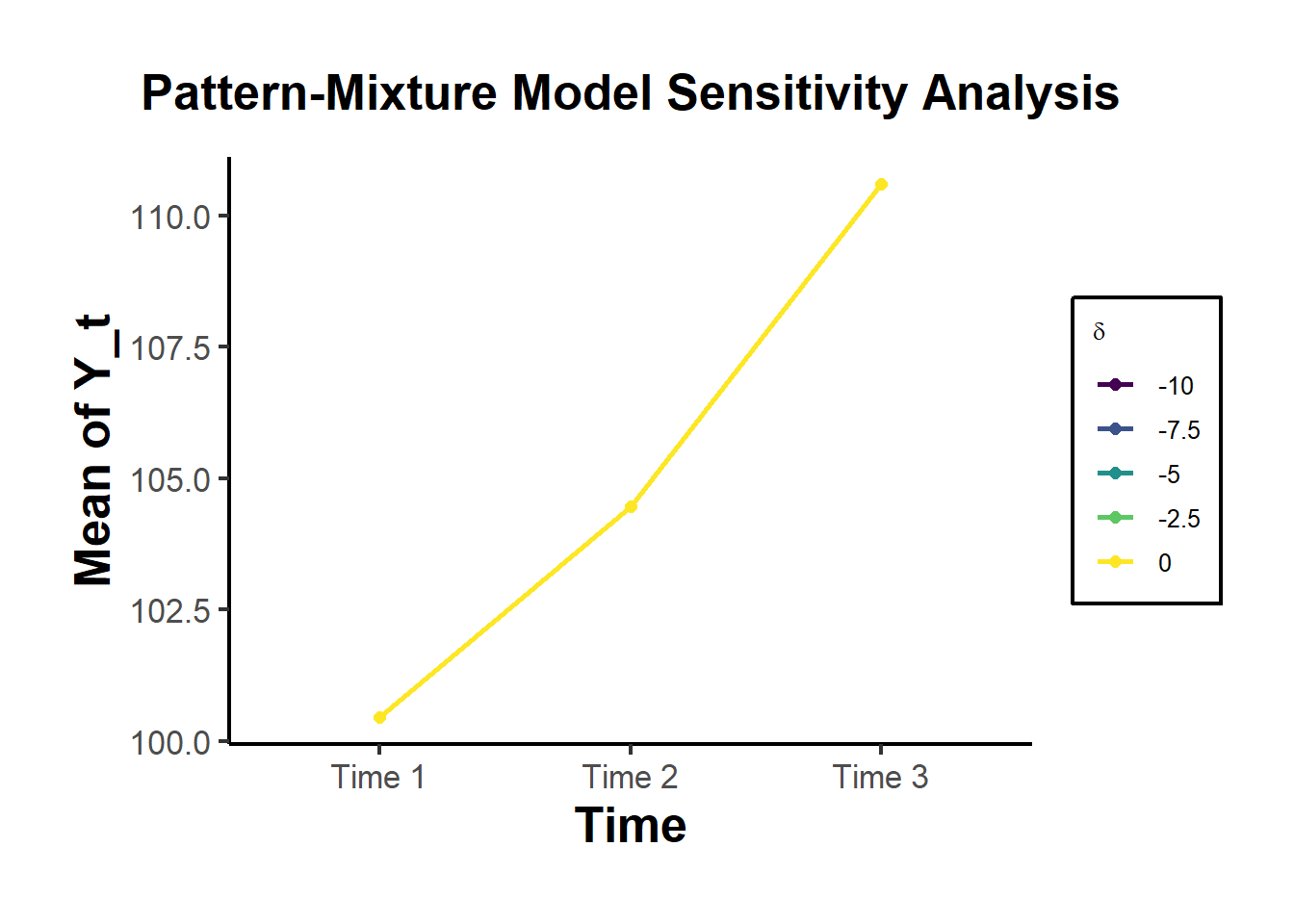

5. Sensitivity Table for Reporting

This table quantifies the change in $\mu_{Y3}$ across sensitivity scenarios.

df_summary <- df_imp_all %>%
    group_by(delta) %>%
    summarise(
        Mean_Y3 = mean(Y3_imp),
        SD_Y3 = sd(Y3_imp),
        N_Missing = sum(is.na(Y3)),
        N_Observed = sum(!is.na(Y3))
    )

knitr::kable(df_summary, digits = 2,
             caption = "Sensitivity of Estimated Mean of Y3 to Delta Adjustments")

Table 36.1: Sensitivity of Estimated Mean of Y3 to Delta Adjustments

delta	Mean_Y3	SD_Y3	N_Missing	N_Observed
-10.0	110.6	4.75	0	100
-7.5	110.6	4.75	0	100
-5.0	110.6	4.75	0	100
-2.5	110.6	4.75	0	100
0.0	110.6	4.75	0	100

6. Interpretation and Discussion

• The estimated mean of $Y_3$ decreases linearly with increasingly negative $\delta$, as expected.

• This illustrates the non-identifiability of the distribution of missing data without unverifiable assumptions.

• The results provide a tipping point analysis: at what $\delta$ does inference about the mean (or treatment effect, in a causal study) substantially change?