19 Mediation
Mediation analysis uncovers the process by which a predictor affects an outcome through one or more intermediate variables. This chapter introduces the traditional approach to mediation, focusing on path analysis, the Baron & Kenny framework, and the Sobel test. Practical limitations of this approach are discussed, especially in the presence of confounding. Then, it presents a modern causal inference framework for mediation, including counterfactual definitions of direct and indirect effects. The use of bootstrapping is demonstrated with business examples. Assumptions such as sequential ignorability are explored in detail. Graphical representations, including path diagrams and causal graphs, are used to aid interpretation. The chapter provides the tools to not only estimate mediation effects but to assess their robustness, interpret their business relevance, and report them transparently.
19.1 Traditional Approach
The classical mediation analysis follows the approach introduced by Baron and Kenny (1986), though it has limitations, particularly in requiring the first step (\(X \to Y\)) to be significant. Despite its shortcomings, this framework provides a useful foundation.
19.1.1 Steps in the Traditional Mediation Model
Mediation is typically assessed through three regression models:
- Total Effect: \(X \to Y\)
- Path \(a\): \(X \to M\)
- Path \(b\) and Direct Effect (\(c'\)): \(X + M \to Y\)
where:
- \(X\) = independent (causal) variable
- \(Y\) = dependent (outcome) variable
- \(M\) = mediating variable
Originally, Baron and Kenny (1986) required the direct path \(X \to Y\) to be significant. However, mediation can still occur even if this direct effect is not significant. For example:
The effect of \(X\) on \(Y\) might be fully absorbed by \(M\).
Multiple mediators (\(M_1, M_2\)) with opposing effects could cancel each other out, leading to a non-significant direct effect.
19.1.2 Graphical Representation of Mediation
19.1.2.1 Unmediated Model
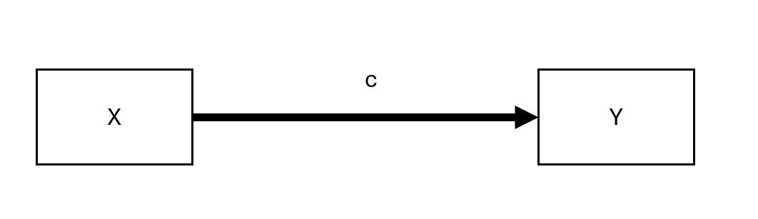
Figure 19.1: Unmediated Model
Here, \(c\) represents the total effect of \(X\) on \(Y\).
19.1.2.2 Mediated Model
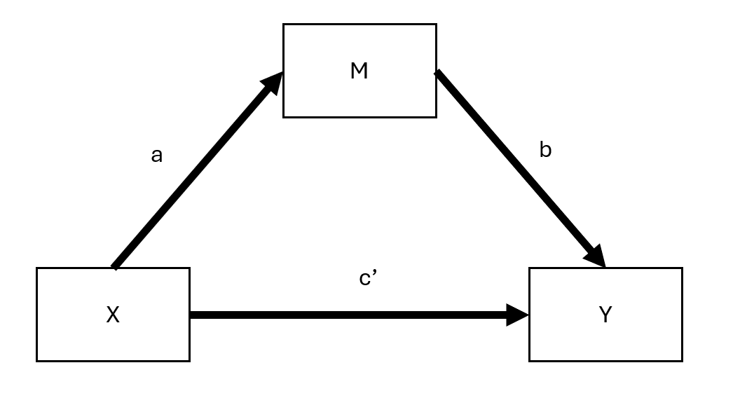
Figure 19.2: Mediated Model
Here:
- \(c'\) = direct effect (effect of \(X\) on \(Y\) after accounting for mediation)
- \(ab\) = indirect effect (mediation pathway)
Thus, we can express:
\[ \text{total effect} = \text{direct effect} + \text{indirect effect} \]
or,
\[ c = c' + ab \]
This equation holds under standard linear models but not necessarily in cases such as:
- Latent variable models
- Logistic regression (only an approximation)
- Multilevel models (Bauer, Preacher, and Gil 2006)
19.1.3 Measuring Mediation
Several approaches exist for quantifying the indirect effect (\(ab\)):
Proportional Reduction Approach:
\[1 - \frac{c'}{c}\]
Not recommended due to high instability, especially when \(c\) is small (D. P. MacKinnon, Warsi, and Dwyer 1995).Product Method:
\[a \times b\]
The most common approach.Difference Method:
\[c - c'\]
Conceptually similar to the product method but less precise in small samples.
19.1.4 Assumptions in Linear Mediation Models
For valid mediation analysis, the following assumptions should hold:
- No unmeasured confounders between \(X-Y\), \(X-M\), and \(M-Y\).
- No reverse causality: \(X\) should not be influenced by a confounder (\(C\)) that also affects \(M-Y\).
- Measurement reliability: \(M\) should be measured without error (if not, consider errors-in-variables models).
Regression Equations for Mediation Steps
Step 1: Total Effect of \(X\) on \(Y\)
\[ Y = \beta_0 + cX + \epsilon \]
- The significance of \(c\) is not required for mediation to occur.
Step 2: Effect of \(X\) on \(M\)
\[ M = \alpha_0 + aX + \epsilon \]
- The coefficient \(a\) must be significant for mediation analysis to proceed.
Step 3: Effect of \(M\) on \(Y\) (Including \(X\))
\[ Y = \gamma_0 + c'X + bM + \epsilon \]
- If \(c'\) becomes non-significant after including \(M\), full mediation occurs.
- If \(c'\) is reduced but remains significant, partial mediation is present.
| Effect of \(X\) on \(Y\) | Mediation Type |
|---|---|
| \(b_4\) (from Step 3) is insignificant | Full mediation |
| \(b_4 < b_1\) (from Step 1) but still significant | Partial mediation |
19.1.5 Testing for Mediation
Several statistical tests exist to assess whether the indirect effect (\(ab\)) is significant:
-
Sobel Test (Sobel 1982)
- Based on the standard error of \(ab\).
- Limitation: Assumes normality of \(ab\), which may not hold in small samples.
-
Joint Significance Test
- If both \(a\) and \(b\) are significant, mediation is likely.
-
Bootstrapping (Preferred) Shrout and Bolger (2002)
- Estimates the confidence interval for \(ab\).
- Does not assume normality.
- Recommended for small-to-moderate sample sizes.
19.1.6 Additional Considerations
- Proximal mediation (where path \(a\) exceeds path \(b\)) can lead to multicollinearity and reduced statistical power. In contrast, distal mediation (where path \(b\) exceeds path \(a\)) tends to maximize power. In fact, slightly distal mediators—where \(b\) is somewhat larger than \(a\)—often strike an ideal balance for power in mediation analyses (Hoyle 1999).
- Tests of direct effects (\(c\) and \(c'\)) generally have lower power than tests of the indirect effect (\(ab\)). As a result, it is possible for the indirect effect (\(ab\)) to be statistically significant even when the direct effect (\(c\)) is not. This situation can appear to indicate “complete mediation,” yet the lack of a statistically significant direct effect between \(X\) and \(Y\) (i.e., \(c'\)) does not definitively rule out other possibilities (Kenny and Judd 2014).
- Because testing \(ab\) essentially combines two tests, it often provides a power advantage over testing \(c'\) alone. However, using a non-significant \(c'\) as the sole criterion for claiming complete mediation should be done cautiously—if at all—given the importance of adequate sample size and power. Indeed, Hayes and Scharkow (2013) recommend avoiding claims of complete mediation based solely on a non-significant \(c'\), particularly when partial mediation may still be present.
19.1.7 Assumptions in Mediation Analysis
Valid mediation analysis requires several key assumptions, which can be categorized into causal direction, interaction effects, measurement reliability, and confounding control.
19.1.7.1 Direction
Causal Order of Variables
A simple but weak solution is to measure \(X\) before \(M\) and \(Y\) to prevent reverse causality (i.e., \(M\) or \(Y\) causing \(X\)). Similarly, measuring \(M\) before \(Y\) avoids feedback effects of \(Y\) on \(M\).
-
However, causal feedback loops between \(M\) and \(Y\) may still exist.
If we assume full mediation (\(c' = 0\)), models with reciprocal causal effects between \(M\) and \(Y\) can be estimated using instrumental variables (IV).
E. R. Smith (1982) suggests treating both \(M\) and \(Y\) as potential mediators of each other, requiring distinct instrumental variables for each to avoid cross-contamination of causal effects.
19.1.7.2 Interaction Effects in Mediation
If \(M\) interacts with \(X\) in predicting \(Y\), then \(M\) is both a mediator and a moderator (Baron and Kenny 1986).
The interaction term \(X \times M\) should always be included in the model to account for possible moderation effects.
For interpreting such interactions in mediation models, see (T. VanderWeele 2015), who provides a framework for moderated mediation analysis.
19.1.7.3 Reliability
Measurement error in any of the three key variables (\(X, M, Y\)) can bias estimates of mediation effects.
- Measurement Error in the Mediator (\(M\)):
- Biases both \(b\) and \(c'\).
- Potential solution: Model \(M\) as a latent variable (reduces bias but may decrease statistical power) (Ledgerwood and Shrout 2011).
- Specific effects:
- \(b\) is attenuated (biased toward 0).
-
\(c'\) is:
- Overestimated if \(ab > 0\).
- Underestimated if \(ab < 0\).
- Measurement Error in the Treatment (\(X\)):
- Biases both \(a\) and \(b\).
- Specific effects:
- \(a\) is attenuated.
-
\(b\) is:
- Overestimated if \(ac' > 0\).
- Underestimated if \(ac' < 0\).
- Measurement Error in the Outcome (\(Y\)):
- If unstandardized, there is no bias.
- If standardized, there is attenuation bias (reduced effect sizes due to error variance).
19.1.7.4 Confounding in Mediation Analysis
Omitted variable bias can distort any of the three core relationships (\(X \to Y\), \(X \to M\), \(M \to Y\)). Addressing confounding requires either design-based or statistical solutions.
Design-Based Strategies (Preferred if Feasible)
- Randomization of the independent variable (\(X\)) reduces confounding bias.
- Randomization of the mediator (\(M\)), if possible, further strengthens causal claims.
- Controlling for measured confounders, though this only addresses observable confounding.
Statistical Strategies (When Randomization is Not Possible)
- Instrumental Variables Approach:
- Used when a confounder affects both \(M\) and \(Y\).
- Front-door adjustment can be applied if there exists a third variable that fully mediates the effect of \(M\) on \(Y\) while being independent of the confounder.
- Weighting Methods (e.g., Inverse Probability Weighting - IPW):
- Corrects for confounding by reweighting observations to balance confounders across treatment groups.
- Requires the strong ignorability assumption: All confounders must be measured and correctly specified (Westfall and Yarkoni 2016).
- While this assumption cannot be formally tested, sensitivity analyses can help assess robustness.
- See Heiss for R code on implementing IPW in mediation models.
19.1.8 Indirect Effect Tests
Testing the indirect effect (\(ab\)) is crucial in mediation analysis. Several methods exist, each with its advantages and limitations.
19.1.8.1 Sobel Test (Delta Method)
- Developed by Sobel (1982).
- Also known as the delta method.
- Not recommended because it assumes the sampling distribution of \(ab\) is normal, which often does not hold (D. P. MacKinnon, Warsi, and Dwyer 1995).
The standard error (SE) of the indirect effect is:
\[ SE_{ab} = \sqrt{\hat{b}^2 s_{\hat{a}}^2 + \hat{a}^2 s_{\hat{b}}^2} \]
The Z-statistic for testing whether \(ab\) is significantly different from 0 is:
\[ z = \frac{\hat{ab}}{\sqrt{\hat{b}^2 s_{\hat{a}}^2 + \hat{a}^2 s_{\hat{b}}^2}} \]
Disadvantages
- Assumes \(a\) and \(b\) are independent.
- Assumes \(ab\) follows a normal distribution.
- Poor performance in small samples.
- Lower power and more conservative than bootstrapping.
Special Case: Inconsistent Mediation
- Mediation can occur even when direct and indirect effects have opposite signs, known as inconsistent mediation (D. P. MacKinnon, Fairchild, and Fritz 2007).
- This happens when the mediator acts as a suppressor variable, leading to counteracting paths.
library(bda)
library(mediation)
data("boundsdata")

# Sobel Test for Mediation
bda::mediation.test(boundsdata$med, boundsdata$ttt, boundsdata$out) |>
    tibble::rownames_to_column() |>
    causalverse::nice_tab(2)
#>   rowname Sobel Aroian Goodman
#> 1 z.value  4.05   4.03    4.07
#> 2 p.value  0.00   0.00    0.00
19.1.8.2 Joint Significance Test
- Tests if the indirect effect is nonzero by checking whether both \(a\) and \(b\) are statistically significant.
- Assumes \(a \perp b\) (independence of paths).
- Performs similarly to bootstrapping (Hayes and Scharkow 2013).
- More robust to non-normality but can be sensitive to heteroscedasticity (Fossum and Montoya 2023).
- Does not provide confidence intervals, making effect size interpretation harder.
19.1.8.3 Bootstrapping (Preferred Method)
- First applied to mediation by Bollen and Stine (1990).
- Uses resampling to empirically estimate the sampling distribution of the indirect effect.
- Does not require normality assumptions or \(a \perp b\) independence.
- Works well with small samples.
- Can handle complex models.
Which Bootstrapping Method?
- Percentile bootstrap is preferred due to better Type I error rates (Tibbe and Montoya 2022).
- Bias-corrected bootstrapping can be too liberal (inflates Type I errors) (Fritz, Taylor, and MacKinnon 2012).
Special Case: Meta-Analytic Bootstrapping
- Bootstrapping can be applied without raw data, using only \(a, b, var(a), var(b), cov(a,b)\) from multiple studies.
# Meta-Analytic Bootstrapping for Mediation
library(causalverse)

result <- causalverse::med_ind(
    a = 0.5,
    b = 0.7,
    var_a = 0.04,
    var_b = 0.05,
    cov_ab = 0.01
)
result$plot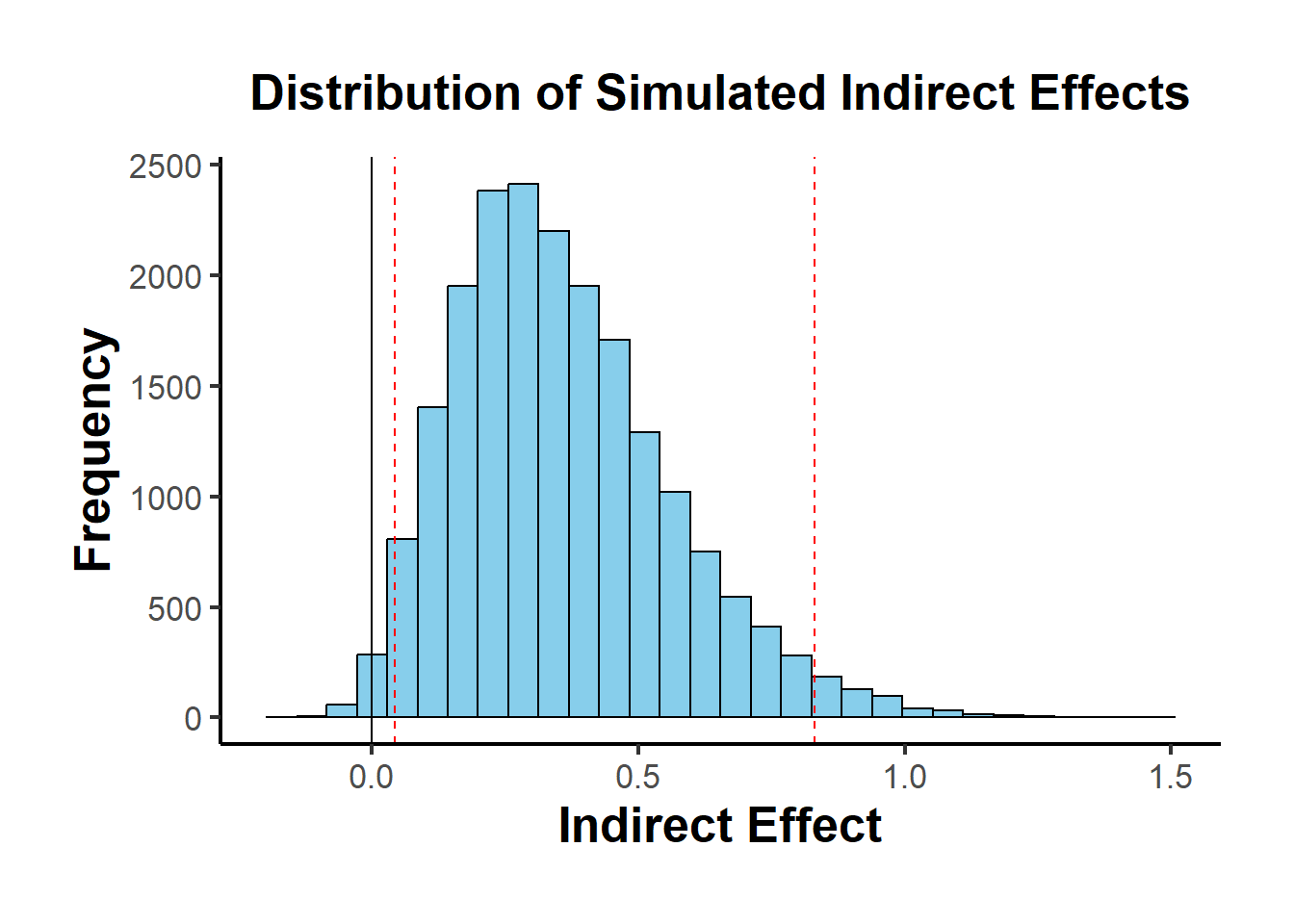
Figure 19.3: Distribution of Simulated Indirect Effects
When an instrumental variable (IV) is available, the causal effect can be estimated more reliably. Below are visual representations.
library(DiagrammeR)

# Simple Treatment-Outcome Model
grViz("
digraph {
  graph []
  node [shape = plaintext]
    X [label = 'Treatment']
    Y [label = 'Outcome']
  edge [minlen = 2]
    X->Y
  { rank = same; X; Y }
}")

# Mediation Model with an Instrument
grViz("
digraph {
  graph []
  node [shape = plaintext]
    X [label ='Treatment', shape = box]
    Y [label ='Outcome', shape = box]
    M [label ='Mediator', shape = box]
    IV [label ='Instrument', shape = box]
  edge [minlen = 2]
    IV->X
    X->M
    M->Y
    X->Y
  { rank = same; X; Y; M }
}")
Mediation Analysis with Fixed Effects Models
library(mediation)
library(fixest)

data("boundsdata")

# Step 1: Total Effect (c)
out1 <- feols(out ~ ttt, data = boundsdata)

# Step 2: Indirect Effect (a)
out2 <- feols(med ~ ttt, data = boundsdata)

# Step 3: Direct & Indirect Effect (c' & b)
out3 <- feols(out ~ med + ttt, data = boundsdata)

# Proportion of Mediation
coef(out2)['ttt'] * coef(out3)['med'] / coef(out1)['ttt'] * 100
#>      ttt
#> 68.63609
Bootstrapped Mediation Analysis
library(boot)
set.seed(1)

# Define the bootstrapping function
mediation_fn <- function(data, i) {
    df <- data[i,]

    a_path <- feols(med ~ ttt, data = df)
    a <- coef(a_path)['ttt']

    b_path <- feols(out ~ med + ttt, data = df)
    b <- coef(b_path)['med']

    cp <- coef(b_path)['ttt']

    # Indirect Effect (a * b)
    ind_ef <- a * b
    total_ef <- a * b + cp
    return(c(ind_ef, total_ef))
}

# Perform Bootstrapping
boot_med <- boot(boundsdata, mediation_fn, R = 100, parallel = "multicore", ncpus = 2)
boot_med
#>
#> ORDINARY NONPARAMETRIC BOOTSTRAP
#>
#>
#> Call:
#> boot(data = boundsdata, statistic = mediation_fn, R = 100, parallel = "multicore",
#>     ncpus = 2)
#>
#>
#> Bootstrap Statistics :
#>       original        bias    std. error
#> t1* 0.04112035  0.0006346725 0.009539903
#> t2* 0.05991068 -0.0004462572 0.029556611

# Summary and Confidence Intervals
summary(boot_med) |> causalverse::nice_tab()
#>     R original bootBias bootSE bootMed
#> 1 100     0.04        0   0.01    0.04
#> 2 100     0.06        0   0.03    0.06

# Confidence Intervals (percentile bootstrap preferred)
boot.ci(boot_med, type = c("norm", "perc"))
#> BOOTSTRAP CONFIDENCE INTERVAL CALCULATIONS
#> Based on 100 bootstrap replicates
#>
#> CALL :
#> boot.ci(boot.out = boot_med, type = c("norm", "perc"))
#>
#> Intervals :
#> Level      Normal             Percentile
#> 95%   ( 0.0218,  0.0592 )   ( 0.0249,  0.0623 )
#> Calculations and Intervals on Original Scale
#> Some percentile intervals may be unstable

# Point Estimates (Indirect and Total Effects)
colMeans(boot_med$t)
#> [1] 0.04175502 0.05946442
Alternatively, use the robmed package for robust mediation analysis:
19.1.9 Power Analysis for Mediation
To assess whether the study has sufficient power to detect mediation effects, use:
library(pwr2ppl)

# Power analysis for the indirect effect (ab path)
medjs(
    rx1m1 = .3,  # Correlation: X → M (path a)
    rx1y  = .1,  # Correlation: X → Y (path c')
    rym1  = .3,  # Correlation: M → Y (path b)
    n     = 100, # Sample size
    alpha = 0.05,
    mvars = 1,   # Number of mediators
    rep   = 1000 # Replications (use 10,000 for accuracy)
)
For interactive power analysis, see Kenny’s Mediation Power App.
Summary of Indirect Effect Tests
| Test | Pros | Cons |
|---|---|---|
| Sobel Test | Simple, fast | Assumes normality, low power |
| Joint Significance Test | Robust to non-normality | No confidence interval |
| Bootstrapping (Recommended) | No normality assumption, handles small samples | May be liberal if bias-corrected |
19.1.10 Multiple Mediation Analysis
In some cases, a single mediator (\(M\)) does not fully capture the indirect effect of \(X\) on \(Y\). Multiple mediation models extend traditional mediation by including two or more mediators, allowing us to examine how multiple pathways contribute to an outcome.
Several R packages handle multiple mediation models:
- manymome: A flexible package for multiple mediation modeling.
-
mma: Used for multiple mediator models.
19.1.10.1 Multiple Mediators: Structural Equation Modeling Approach
A popular method for estimating multiple mediation models is Structural Equation Modeling using lavaan.
To test multiple mediation, we first simulate data where two mediators (\(M_1\) and \(M_2\)) contribute to the outcome (\(Y\)).
# Load required packages
library(MASS)  # For mvrnorm (generating correlated errors)
library(lavaan)

# Function to generate synthetic data
generate_data <- function(n = 10000, a1 = 0.5, a2 = -0.35,
                          b1 = 0.7, b2 = 0.48,
                          corr = TRUE, correlation_value = 0.7) {
    set.seed(12345)
    X <- rnorm(n)  # Independent variable

    # Generate correlated errors for mediators
    if (corr) {
        Sigma <- matrix(c(1, correlation_value, correlation_value, 1), nrow = 2)
        errors <- mvrnorm(n, mu = c(0, 0), Sigma = Sigma)
    } else {
        errors <- mvrnorm(n, mu = c(0, 0), Sigma = diag(2))
    }

    M1 <- a1 * X + errors[, 1]
    M2 <- a2 * X + errors[, 2]
    Y  <- b1 * M1 + b2 * M2 + rnorm(n)  # Outcome variable

    return(data.frame(X = X, M1 = M1, M2 = M2, Y = Y))
}
We analyze the indirect effects through both mediators (\(M_1\) and \(M_2\)).
- Correctly Modeling Correlated Mediators
# Generate data with correlated mediators
Data_corr <- generate_data(n = 10000, corr = TRUE, correlation_value = 0.7)

# Define SEM model for multiple mediation
model_corr <- '
  Y ~ b1 * M1 + b2 * M2 + c * X
  M1 ~ a1 * X
  M2 ~ a2 * X
  M1 ~~ M2  # Correlated mediators (modeling correlation correctly)
'

# Fit SEM model
fit_corr <- sem(model_corr, data = Data_corr)

# Extract parameter estimates
parameterEstimates(fit_corr)[, c("lhs", "rhs", "est", "se", "pvalue")]
#>    lhs rhs    est    se pvalue
#> 1    Y  M1  0.700 0.014  0.000
#> 2    Y  M2  0.487 0.014  0.000
#> 3    Y   X -0.009 0.015  0.545
#> 4   M1   X  0.519 0.010  0.000
#> 5   M2   X -0.340 0.010  0.000
#> 6   M1  M2  0.677 0.012  0.000
#> 7    Y   Y  0.975 0.014  0.000
#> 8   M1  M1  0.973 0.014  0.000
#> 9   M2  M2  0.982 0.014  0.000
#> 10   X   X  1.000 0.000     NA
2. Incorrectly Ignoring Correlation Between Mediators
# Define SEM model without modeling mediator correlation
model_uncorr <- '
  Y ~ b1 * M1 + b2 * M2 + c * X
  M1 ~ a1 * X
  M2 ~ a2 * X
'

# Fit incorrect model
fit_uncorr <- sem(model_uncorr, data = Data_corr)

# Compare parameter estimates
parameterEstimates(fit_uncorr)[, c("lhs", "rhs", "est", "se", "pvalue")]
#>   lhs rhs    est    se pvalue
#> 1   Y  M1  0.700 0.010  0.000
#> 2   Y  M2  0.487 0.010  0.000
#> 3   Y   X -0.009 0.012  0.443
#> 4  M1   X  0.519 0.010  0.000
#> 5  M2   X -0.340 0.010  0.000
#> 6   Y   Y  0.975 0.014  0.000
#> 7  M1  M1  0.973 0.014  0.000
#> 8  M2  M2  0.982 0.014  0.000
#> 9   X   X  1.000 0.000     NA
Comparison of Model Fits
To check whether modeling correlation matters, we compare AIC and RMSEA.
# Extract model fit statistics
fit_measures <- function(fit) {
  fitMeasures(fit, c("aic", "bic", "rmsea", "chisq"))
}

# Compare model fits
fit_measures(fit_corr)  # Correct model (correlated mediators)
#>      aic      bic    rmsea    chisq
#> 77932.45 77997.34     0.00     0.00
fit_measures(fit_uncorr)  # Incorrect model (ignores correlation)
#>       aic       bic     rmsea     chisq
#> 84453.208 84510.891 0.808 6522.762- If AIC and RMSEA are lower in the correlated model, it suggests that accounting for correlated errors improves fit.
After fitting the model, we assess:
Direct Effect: The effect of \(X\) on \(Y\) after accounting for both mediators (\(c'\)).
-
Indirect Effects:
\(a_1 \times b_1\): Effect of \(X \to M_1 \to Y\).
\(a_2 \times b_2\): Effect of \(X \to M_2 \to Y\).
Total Effect: Sum of direct and indirect effects.
# Extract indirect and direct effects
parameterEstimates(fit_corr, standardized = TRUE)
#>    lhs op rhs label    est    se       z pvalue ci.lower ci.upper std.lv
#> 1    Y  ~  M1    b1  0.700 0.014  50.489  0.000    0.673    0.727  0.700
#> 2    Y  ~  M2    b2  0.487 0.014  35.284  0.000    0.460    0.514  0.487
#> 3    Y  ~   X     c -0.009 0.015  -0.606  0.545   -0.038    0.020 -0.009
#> 4   M1  ~   X    a1  0.519 0.010  52.563  0.000    0.499    0.538  0.519
#> 5   M2  ~   X    a2 -0.340 0.010 -34.314  0.000   -0.360   -0.321 -0.340
#> 6   M1 ~~  M2        0.677 0.012  56.915  0.000    0.654    0.700  0.677
#> 7    Y ~~   Y        0.975 0.014  70.711  0.000    0.948    1.002  0.975
#> 8   M1 ~~  M1        0.973 0.014  70.711  0.000    0.946    1.000  0.973
#> 9   M2 ~~  M2        0.982 0.014  70.711  0.000    0.955    1.010  0.982
#> 10   X ~~   X        1.000 0.000      NA     NA    1.000    1.000  1.000
#>    std.all std.nox
#> 1    0.528   0.528
#> 2    0.345   0.345
#> 3   -0.006  -0.006
#> 4    0.465   0.465
#> 5   -0.325  -0.325
#> 6    0.692   0.692
#> 7    0.447   0.447
#> 8    0.784   0.784
#> 9    0.895   0.895
#> 10   1.000   1.000
If \(c'\) is reduced (but still significant), we have partial mediation. If \(c' \approx 0\), it suggests full mediation.
# Load required packages
library(MASS)  # for mvrnorm
library(lavaan)

# Function to generate synthetic data with correctly correlated errors for mediators
generate_data <-
  function(n = 10000,
           a1 = 0.5,
           a2 = -0.35,
           b1 = 0.7,
           b2 = 0.48,
           corr = TRUE,
           correlation_value = 0.7) {
    set.seed(12345)
    X <- rnorm(n)

    # Generate correlated errors using a multivariate normal distribution
    if (corr) {
        Sigma <- matrix(c(1, correlation_value, correlation_value, 1), nrow = 2)  # Higher covariance matrix for errors
        errors <- mvrnorm(n, mu = c(0, 0), Sigma = Sigma)  # Generate correlated errors
    } else {
        errors <- mvrnorm(n, mu = c(0, 0), Sigma = diag(2))  # Independent errors
    }

    M1 <- a1 * X + errors[, 1]
    M2 <- a2 * X + errors[, 2]
    Y <- b1 * M1 + b2 * M2 + rnorm(n)  # Y depends on M1 and M2

    data.frame(X = X, M1 = M1, M2 = M2, Y = Y)
}

# Ground truth for comparison
ground_truth <- data.frame(Parameter = c("b1", "b2"), GroundTruth = c(0.7, 0.48))

# Function to extract relevant estimates, standard errors, and model fit
extract_estimates_b1_b2 <- function(fit) {
    estimates <- parameterEstimates(fit)
    estimates <- estimates[estimates$lhs == "Y" & estimates$rhs %in% c("M1", "M2"), c("rhs", "est", "se")]
    estimates$Parameter <- ifelse(estimates$rhs == "M1", "b1", "b2")
    estimates <- estimates[, c("Parameter", "est", "se")]
    fit_stats <- fitMeasures(fit, c("aic", "bic", "rmsea", "chisq"))
    return(list(estimates = estimates, fit_stats = fit_stats))
}

# Case 1: Correlated errors for mediators (modeled correctly)
Data_corr <- generate_data(n = 10000, corr = TRUE, correlation_value = 0.7)
model_corr <- '
  Y ~ b1 * M1 + b2 * M2 + c * X
  M1 ~ a1 * X
  M2 ~ a2 * X
  M1 ~~ M2  # Correlated mediators (errors)
'
fit_corr <- sem(model = model_corr, data = Data_corr)
results_corr <- extract_estimates_b1_b2(fit_corr)

# Case 2: Uncorrelated errors for mediators (modeled correctly)
Data_uncorr <- generate_data(n = 10000, corr = FALSE)
model_uncorr <- '
  Y ~ b1 * M1 + b2 * M2 + c * X
  M1 ~ a1 * X
  M2 ~ a2 * X
'
fit_uncorr <- sem(model = model_uncorr, data = Data_uncorr)
results_uncorr <- extract_estimates_b1_b2(fit_uncorr)

# Case 3: Correlated errors, but not modeled as correlated
fit_corr_incorrect <- sem(model = model_uncorr, data = Data_corr)
results_corr_incorrect <- extract_estimates_b1_b2(fit_corr_incorrect)

# Case 4: Uncorrelated errors, but modeled as correlated
fit_uncorr_incorrect <- sem(model = model_corr, data = Data_uncorr)
results_uncorr_incorrect <- extract_estimates_b1_b2(fit_uncorr_incorrect)

# Combine all estimates for comparison
estimates_combined <- list(
    "Correlated (Correct)" = results_corr$estimates,
    "Uncorrelated (Correct)" = results_uncorr$estimates,
    "Correlated (Incorrect)" = results_corr_incorrect$estimates,
    "Uncorrelated (Incorrect)" = results_uncorr_incorrect$estimates
)

# Combine all into a single table
comparison_table <- do.call(rbind, lapply(names(estimates_combined), function(case) {
    df <- estimates_combined[[case]]
    df$Case <- case
    df
}))

# Merge with ground truth for final comparison
comparison_table <- merge(comparison_table, ground_truth, by = "Parameter")

# Display the comparison table
comparison_table
#>   Parameter       est          se                     Case GroundTruth
#> 1        b1 0.7002984 0.013870433     Correlated (Correct)        0.70
#> 2        b1 0.6973612 0.009859426   Uncorrelated (Correct)        0.70
#> 3        b1 0.7002984 0.010010367   Correlated (Incorrect)        0.70
#> 4        b1 0.6973612 0.009859634 Uncorrelated (Incorrect)        0.70
#> 5        b2 0.4871118 0.013805615     Correlated (Correct)        0.48
#> 6        b2 0.4868318 0.010009908   Uncorrelated (Correct)        0.48
#> 7        b2 0.4871118 0.009963588   Correlated (Incorrect)        0.48
#> 8        b2 0.4868318 0.010010119 Uncorrelated (Incorrect)        0.48

# Display model fit statistics for each case
fit_stats_combined <- list(
    "Correlated (Correct)" = results_corr$fit_stats,
    "Uncorrelated (Correct)" = results_uncorr$fit_stats,
    "Correlated (Incorrect)" = results_corr_incorrect$fit_stats,
    "Uncorrelated (Incorrect)" = results_uncorr_incorrect$fit_stats
)

fit_stats_combined
#> $`Correlated (Correct)`
#>      aic      bic    rmsea    chisq
#> 77932.45 77997.34     0.00     0.00
#>
#> $`Uncorrelated (Correct)`
#>       aic       bic     rmsea     chisq
#> 84664.312 84721.995     0.000     0.421
#>
#> $`Correlated (Incorrect)`
#>       aic       bic     rmsea     chisq
#> 84453.208 84510.891     0.808  6522.762
#>
#> $`Uncorrelated (Incorrect)`
#>      aic      bic    rmsea    chisq
#> 84665.89 84730.78     0.00     0.00
19.1.11 Multiple Treatments in Mediation
In some cases, multiple independent variables (\(X_1\), \(X_2\)) influence the same mediators. This is called multiple treatments mediation (Hayes and Preacher 2014).
For an example in PROCESS (SPSS/R), see:
Process Mediation with Multiple Treatments.
19.2 Causal Inference Approach to Mediation
Traditional mediation models assume that regression-based estimates provide valid causal inference. However, causal mediation analysis (CMA) extends beyond traditional models by explicitly defining mediation in terms of potential outcomes and counterfactuals.
19.2.1 Example: Traditional Mediation Analysis
We begin with a classic three-step mediation approach.
# Load data
myData <- read.csv("data/mediationData.csv")

# Step 1 (Total Effect: X → Y) [No longer required]
model.0 <- lm(Y ~ X, data = myData)
summary(model.0)
#>
#> Call:
#> lm(formula = Y ~ X, data = myData)
#>
#> Residuals:
#>     Min      1Q  Median      3Q     Max
#> -5.0262 -1.2340 -0.3282  1.5583  5.1622
#>
#> Coefficients:
#>             Estimate Std. Error t value Pr(>|t|)
#> (Intercept)   2.8572     0.6932   4.122 7.88e-05 ***
#> X             0.3961     0.1112   3.564 0.000567 ***
#> ---
#> Signif. codes:  0 '***' 0.001 '**' 0.01 '*' 0.05 '.' 0.1 ' ' 1
#>
#> Residual standard error: 1.929 on 98 degrees of freedom
#> Multiple R-squared:  0.1147, Adjusted R-squared:  0.1057
#> F-statistic:  12.7 on 1 and 98 DF,  p-value: 0.0005671

# Step 2 (Effect of X on M)
model.M <- lm(M ~ X, data = myData)
summary(model.M)
#>
#> Call:
#> lm(formula = M ~ X, data = myData)
#>
#> Residuals:
#>     Min      1Q  Median      3Q     Max
#> -4.3046 -0.8656  0.1344  1.1344  4.6954
#>
#> Coefficients:
#>             Estimate Std. Error t value Pr(>|t|)
#> (Intercept)  1.49952    0.58920   2.545   0.0125 *
#> X            0.56102    0.09448   5.938 4.39e-08 ***
#> ---
#> Signif. codes:  0 '***' 0.001 '**' 0.01 '*' 0.05 '.' 0.1 ' ' 1
#>
#> Residual standard error: 1.639 on 98 degrees of freedom
#> Multiple R-squared:  0.2646, Adjusted R-squared:  0.2571
#> F-statistic: 35.26 on 1 and 98 DF,  p-value: 4.391e-08

# Step 3 (Effect of M on Y, controlling for X)
model.Y <- lm(Y ~ X + M, data = myData)
summary(model.Y)
#>
#> Call:
#> lm(formula = Y ~ X + M, data = myData)
#>
#> Residuals:
#>     Min      1Q  Median      3Q     Max
#> -3.7631 -1.2393  0.0308  1.0832  4.0055
#>
#> Coefficients:
#>             Estimate Std. Error t value Pr(>|t|)
#> (Intercept)   1.9043     0.6055   3.145   0.0022 **
#> X             0.0396     0.1096   0.361   0.7187
#> M             0.6355     0.1005   6.321 7.92e-09 ***
#> ---
#> Signif. codes:  0 '***' 0.001 '**' 0.01 '*' 0.05 '.' 0.1 ' ' 1
#>
#> Residual standard error: 1.631 on 97 degrees of freedom
#> Multiple R-squared:  0.373,  Adjusted R-squared:  0.3601
#> F-statistic: 28.85 on 2 and 97 DF,  p-value: 1.471e-10

# Step 4: Bootstrapping for ACME
library(mediation)
results <-
    mediate(
        model.M,
        model.Y,
        treat = 'X',
        mediator = 'M',
        boot = TRUE,
        sims = 500
    )
summary(results)
#>
#> Causal Mediation Analysis
#>
#> Nonparametric Bootstrap Confidence Intervals with the Percentile Method
#>
#>                 Estimate 95% CI Lower 95% CI Upper p-value
#> ACME            0.356522     0.211871     0.507799  <2e-16 ***
#> ADE             0.039604    -0.174982     0.278427   0.760
#> Total Effect    0.396126     0.174283     0.643540   0.004 **
#> Prop. Mediated  0.900022     0.504160     1.937520   0.004 **
#> ---
#> Signif. codes:  0 '***' 0.001 '**' 0.01 '*' 0.05 '.' 0.1 ' ' 1
#>
#> Sample Size Used: 100
#>
#>
#> Simulations: 500- Total Effect: \(\hat{c} = 0.3961\) → effect of \(X\) on \(Y\) without controlling for \(M\).
- Direct Effect (ADE): \(\hat{c'} = 0.0396\) → effect of \(X\) on \(Y\) after accounting for \(M\).
-
ACME (Average Causal Mediation Effect):
ACME = \(\hat{c} - \hat{c'} = 0.3961 - 0.0396 = 0.3565\)
Equivalent to product of paths: \(\hat{a} \times \hat{b} = 0.56102 \times 0.6355 = 0.3565\).
These calculations do not rely on strong causal assumptions. For a causal interpretation, we need a more rigorous framework.
19.2.2 Two Approaches in Causal Mediation Analysis
The mediation package Imai, Keele, and Yamamoto (2010) enables causal mediation analysis. It supports two inference types:
-
Model-Based Inference
-
Assumptions:
Treatment is randomized (or approximated via matching).
-
Sequential Ignorability: No unobserved confounding in:
Treatment → Mediator
Treatment → Outcome
Mediator → Outcome
This assumption is hard to justify in observational studies.
-
-
Design-Based Inference
- Relies on experimental design to isolate the causal mechanism.
Notation
We follow the standard potential outcomes framework:
\(M_i(t)\) = mediator under treatment condition \(t\)
\(T_i \in {0,1}\) = treatment assignment
\(Y_i(t, m)\) = outcome under treatment \(t\) and mediator value \(m\)
\(X_i\) = observed pre-treatment covariates
The treatment effect for an individual \(i\): \[ \tau_i = Y_i(1,M_i(1)) - Y_i (0,M_i(0)) \] which decomposes into:
- Causal Mediation Effect (ACME):
\[ \delta_i (t) = Y_i (t,M_i(1)) - Y_i(t,M_i(0)) \]
- Direct Effect (ADE):
\[ \zeta_i (t) = Y_i (1, M_i(1)) - Y_i(0, M_i(0)) \]
Summing up:
\[ \tau_i = \delta_i (t) + \zeta_i (1-t) \]
Sequential Ignorability Assumption
For CMA to be valid, we assume:
\[ \begin{aligned} \{ Y_i (t', m), M_i (t) \} &\perp T_i |X_i = x\\ Y_i(t',m) &\perp M_i(t) | T_i = t, X_i = x \end{aligned} \]
First condition is the standard strong ignorability condition where treatment assignment is random conditional on pre-treatment confounders.
Second condition is stronger where the mediators is also random given the observed treatment and pre-treatment confounders. This condition is satisfied only when there is no unobserved pre-treatment confounders, and post-treatment confounders, and multiple mediators that are correlated.
Key Challenge
Sequential Ignorability is not testable. Researchers should conduct sensitivity analysis.
We now fit a causal mediation model using mediation.
library(mediation)
set.seed(2014)
data("framing", package = "mediation")

# Step 1: Fit mediator model (M ~ T, X)
med.fit <-
    lm(emo ~ treat + age + educ + gender + income, data = framing)

# Step 2: Fit outcome model (Y ~ M, T, X)
out.fit <-
    glm(
        cong_mesg ~ emo + treat + age + educ + gender + income,
        data = framing,
        family = binomial("probit")
    )

# Step 3: Causal Mediation Analysis (Quasi-Bayesian)
med.out <-
    mediate(
        med.fit,
        out.fit,
        treat = "treat",
        mediator = "emo",
        robustSE = TRUE,
        sims = 100
    )  # Use sims = 10000 in practice
summary(med.out)
#>
#> Causal Mediation Analysis
#>
#> Quasi-Bayesian Confidence Intervals
#>
#>                           Estimate 95% CI Lower 95% CI Upper p-value
#> ACME (control)            0.079128     0.035058     0.150095  <2e-16 ***
#> ACME (treated)            0.080385     0.036654     0.155707  <2e-16 ***
#> ADE (control)             0.020551    -0.097597     0.115775    0.70
#> ADE (treated)             0.021808    -0.105256     0.122624    0.70
#> Total Effect              0.100936    -0.049706     0.233869    0.14
#> Prop. Mediated (control)  0.694620    -6.310861     3.679318    0.14
#> Prop. Mediated (treated)  0.711848    -5.793642     3.496550    0.14
#> ACME (average)            0.079756     0.035856     0.153702  <2e-16 ***
#> ADE (average)             0.021180    -0.101427     0.119199    0.70
#> Prop. Mediated (average)  0.703234    -6.052251     3.587934    0.14
#> ---
#> Signif. codes:  0 '***' 0.001 '**' 0.01 '*' 0.05 '.' 0.1 ' ' 1
#>
#> Sample Size Used: 265
#>
#>
#> Simulations: 100
Alternative: Nonparametric Bootstrap
med.out <-
    mediate(
        med.fit,
        out.fit,
        boot = TRUE,
        treat = "treat",
        mediator = "emo",
        sims = 100,
        boot.ci.type = "bca"
    )
summary(med.out)
#>
#> Causal Mediation Analysis
#>
#> Nonparametric Bootstrap Confidence Intervals with the BCa Method
#>
#>                            Estimate 95% CI Lower 95% CI Upper p-value
#> ACME (control)             0.084786     0.042409     0.135927  <2e-16 ***
#> ACME (treated)             0.085820     0.041012     0.136296  <2e-16 ***
#> ADE (control)              0.011654    -0.072556     0.133438    0.58
#> ADE (treated)              0.012689    -0.078400     0.141850    0.58
#> Total Effect               0.097475     0.012219     0.249860    0.06 .
#> Prop. Mediated (control)   0.869822     1.746034   151.198626    0.06 .
#> Prop. Mediated (treated)   0.880437     1.687950   138.906093    0.06 .
#> ACME (average)             0.085303     0.043380     0.137194  <2e-16 ***
#> ADE (average)              0.012172    -0.075578     0.137570    0.58
#> Prop. Mediated (average)   0.875130     1.716992   145.052358    0.06 .
#> ---
#> Signif. codes:  0 '***' 0.001 '**' 0.01 '*' 0.05 '.' 0.1 ' ' 1
#>
#> Sample Size Used: 265
#>
#>
#> Simulations: 100
If we suspect moderation, we include an interaction term.
med.fit <-
    lm(emo ~ treat + age + educ + gender + income, data = framing)

out.fit <-
    glm(
        cong_mesg ~ emo * treat + age + educ + gender + income,
        data = framing,
        family = binomial("probit")
    )

med.out <-
    mediate(
        med.fit,
        out.fit,
        treat = "treat",
        mediator = "emo",
        robustSE = TRUE,
        sims = 100
    )

summary(med.out)
#>
#> Causal Mediation Analysis
#>
#> Quasi-Bayesian Confidence Intervals
#>
#>                             Estimate 95% CI Lower 95% CI Upper p-value
#> ACME (control)             0.0741675    0.0240117    0.1364901  <2e-16 ***
#> ACME (treated)             0.0949636    0.0270237    0.1630112  <2e-16 ***
#> ADE (control)             -0.0135332   -0.1185510    0.1096060    0.76
#> ADE (treated)              0.0072629   -0.1100691    0.1145408    0.90
#> Total Effect               0.0814304   -0.0564589    0.1924589    0.26
#> Prop. Mediated (control)   0.6451040  -14.3124300    3.1336595    0.26
#> Prop. Mediated (treated)   0.9800632  -17.8320223    4.0060277    0.26
#> ACME (average)             0.0845655    0.0273792    0.1470397  <2e-16 ***
#> ADE (average)             -0.0031352   -0.1145684    0.1172708    1.00
#> Prop. Mediated (average)   0.8125836  -16.0722261    3.5478494    0.26
#> ---
#> Signif. codes:  0 '***' 0.001 '**' 0.01 '*' 0.05 '.' 0.1 ' ' 1
#>
#> Sample Size Used: 265
#>
#>
#> Simulations: 100
test.TMint(med.out, conf.level = .95)  # Tests for interaction effect
#>
#>  Test of ACME(1) - ACME(0) = 0
#>
#> data:  estimates from med.out
#> ACME(1) - ACME(0) = 0.020796, p-value = 0.3
#> alternative hypothesis: true ACME(1) - ACME(0) is not equal to 0
#> 95 percent confidence interval:
#>  -0.01757310  0.07110837
Since sequential ignorability is untestable, we examine how unmeasured confounding affects ACME estimates.
# Load required package
library(mediation)

# Simulate some example data
set.seed(123)
n <- 100
data <- data.frame(
  treat = rbinom(n, 1, 0.5),       # Binary treatment
  med = rnorm(n),                   # Continuous mediator
  outcome = rnorm(n)                 # Continuous outcome
)

# Fit the mediator model (med ~ treat)
med_model <- lm(med ~ treat, data = data)

# Fit the outcome model (outcome ~ treat + med)
outcome_model <- lm(outcome ~ treat + med, data = data)

# Perform mediation analysis
med_out <- mediate(med_model,
                   outcome_model,
                   treat = "treat",
                   mediator = "med",
                   sims = 100)

# Conduct sensitivity analysis
sens_out <- medsens(med_out, sims = 100)

summary(sens_out)
#>
#> Mediation Sensitivity Analysis for Average Causal Mediation Effect
#>
#> Sensitivity Region
#>
#>        Rho    ACME 95% CI Lower 95% CI Upper R^2_M*R^2_Y* R^2_M~R^2_Y~
#>  [1,] -0.9 -0.6194      -1.3431       0.1043         0.81       0.7807
#>  [2,] -0.8 -0.3898      -0.8479       0.0682         0.64       0.6168
#>  [3,] -0.7 -0.2790      -0.6096       0.0516         0.49       0.4723
#>  [4,] -0.6 -0.2067      -0.4552       0.0418         0.36       0.3470
#>  [5,] -0.5 -0.1525      -0.3406       0.0355         0.25       0.2409
#>  [6,] -0.4 -0.1083      -0.2487       0.0321         0.16       0.1542
#>  [7,] -0.3 -0.0700      -0.1723       0.0323         0.09       0.0867
#>  [8,] -0.2 -0.0354      -0.1097       0.0389         0.04       0.0386
#>  [9,] -0.1 -0.0028      -0.0648       0.0591         0.01       0.0096
#> [10,]  0.0  0.0287      -0.0416       0.0990         0.00       0.0000
#> [11,]  0.1  0.0603      -0.0333       0.1538         0.01       0.0096
#> [12,]  0.2  0.0928      -0.0317       0.2173         0.04       0.0386
#> [13,]  0.3  0.1275      -0.0333       0.2882         0.09       0.0867
#> [14,]  0.4  0.1657      -0.0369       0.3684         0.16       0.1542
#> [15,]  0.5  0.2100      -0.0422       0.4621         0.25       0.2409
#> [16,]  0.6  0.2642      -0.0495       0.5779         0.36       0.3470
#> [17,]  0.7  0.3364      -0.0601       0.7329         0.49       0.4723
#> [18,]  0.8  0.4473      -0.0771       0.9717         0.64       0.6168
#> [19,]  0.9  0.6768      -0.1135       1.4672         0.81       0.7807
#>
#> Rho at which ACME = 0: -0.1
#> R^2_M*R^2_Y* at which ACME = 0: 0.01
#> R^2_M~R^2_Y~ at which ACME = 0: 0.0096
plot(sens_out)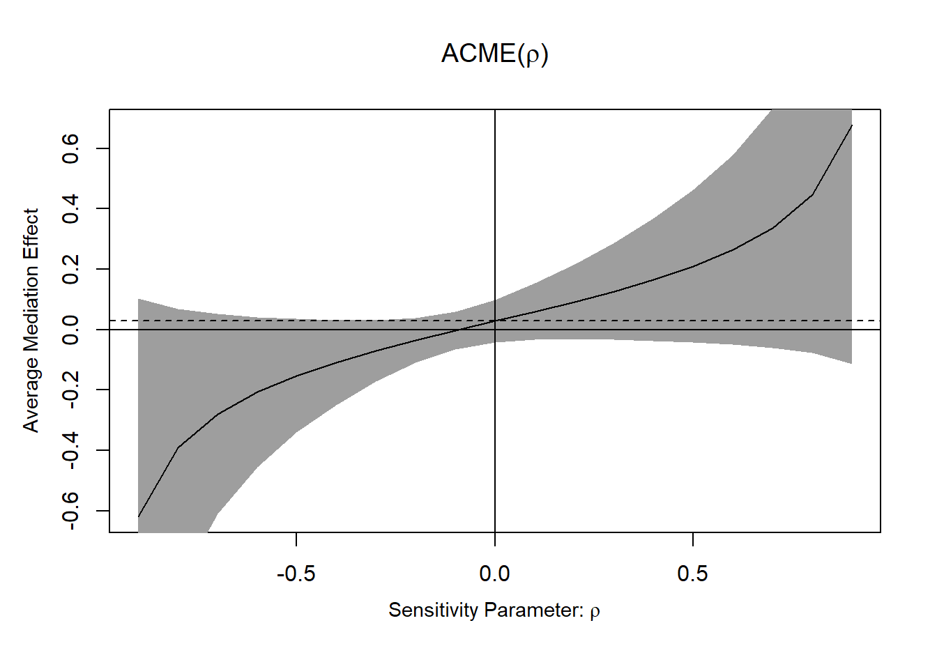
Figure 19.4: ACME
- If ACME confidence intervals contain 0, the effect is not robust to confounding.
Alternatively, using \(R^2\) interpretation, we need to specify the direction of confounder that affects the mediator and outcome variables in plot using sign.prod = "positive" (i.e., same direction) or sign.prod = "negative" (i.e., opposite direction).
plot(sens.out, sens.par = "R2", r.type = "total", sign.prod = "positive")| Aspect | Traditional Mediation | Causal Mediation |
|---|---|---|
| Model Assumption | Linear regressions | Potential outcomes framework |
| Assumptions Needed | No omitted confounders | Sequential ignorability |
| Inference Method | Product of coefficients | Counterfactual reasoning |
| Bootstrapping? | Common | Essential |
| Sensitivity Analysis? | Rarely used | Strongly recommended |