2 Prerequisites
This chapter reviews essential mathematical and computational tools required for effective statistical analysis. Beginning with Matrix Theory and core concepts in linear algebra, we then explore foundational Probability Theory, including random variables, distributions, and expectations. The chapter also revisits important mathematical skills—such as functions, derivatives, and logarithms—before moving into practical elements like data import/export and data manipulation using R. These topics ensure that readers are well-equipped to tackle the more advanced statistical methods presented in later chapters.
If you are confident in your understanding of these topics, you can proceed directly to the Descriptive Statistics section to begin exploring applied data analysis.
2.1 Matrix Theory
Matrix \(A\) represents the original matrix. It’s a 2x2 matrix with elements \(a_{ij}\), where \(i\) represents the row and \(j\) represents the column.
\[ A = \begin{bmatrix} a_{11} & a_{12} \\ a_{21} & a_{22} \end{bmatrix} \]
\(A'\) is the transpose of \(A\). The transpose of a matrix flips its rows and columns.
\[ A' = \begin{bmatrix} a_{11} & a_{21} \\ a_{12} & a_{22} \end{bmatrix} \]
Fundamental properties and rules of matrices, essential for understanding operations in linear algebra:
\[ \begin{aligned} \mathbf{(ABC)'} & = \mathbf{C'B'A'} \quad &\text{(Transpose reverses order in a product)} \\ \mathbf{A(B+C)} & = \mathbf{AB + AC} \quad &\text{(Distributive property)} \\ \mathbf{AB} & \neq \mathbf{BA} \quad &\text{(Multiplication is not commutative)} \\ \mathbf{(A')'} & = \mathbf{A} \quad &\text{(Double transpose is the original matrix)} \\ \mathbf{(A+B)'} & = \mathbf{A' + B'} \quad &\text{(Transpose of a sum is the sum of transposes)} \\ \mathbf{(AB)'} & = \mathbf{B'A'} \quad &\text{(Transpose reverses order in a product)} \\ \mathbf{(AB)^{-1}} & = \mathbf{B^{-1}A^{-1}} \quad &\text{(Inverse reverses order in a product)} \\ \mathbf{A+B} & = \mathbf{B + A} \quad &\text{(Addition is commutative)} \\ \mathbf{AA^{-1}} & = \mathbf{I} \quad &\text{(Matrix times its inverse is identity)} \end{aligned} \]
These properties are critical in solving systems of equations, optimizing models, and performing data transformations.
If a matrix \(\mathbf{A}\) has an inverse, it is called invertible. If \(\mathbf{A}\) does not have an inverse, it is referred to as singular.
The product of two matrices \(\mathbf{A}\) and \(\mathbf{B}\) is computed as:
\[ \begin{aligned} \mathbf{A} &= \begin{bmatrix} a_{11} & a_{12} & a_{13} \\ a_{21} & a_{22} & a_{23} \end{bmatrix} \begin{bmatrix} b_{11} & b_{12} & b_{13} \\ b_{21} & b_{22} & b_{23} \\ b_{31} & b_{32} & b_{33} \end{bmatrix} \\ &= \begin{bmatrix} a_{11}b_{11}+a_{12}b_{21}+a_{13}b_{31} & \sum_{i=1}^{3}a_{1i}b_{i2} & \sum_{i=1}^{3}a_{1i}b_{i3} \\ \sum_{i=1}^{3}a_{2i}b_{i1} & \sum_{i=1}^{3}a_{2i}b_{i2} & \sum_{i=1}^{3}a_{2i}b_{i3} \end{bmatrix} \end{aligned} \]
Quadratic Form
Let \(\mathbf{a}\) be a \(3 \times 1\) vector. The quadratic form involving a matrix \(\mathbf{B}\) is given by:
\[ \mathbf{a'Ba} = \sum_{i=1}^{3}\sum_{j=1}^{3}a_i b_{ij} a_{j} \]
Length of a Vector
The length (or 2-norm) of a vector \(\mathbf{a}\), denoted as \(||\mathbf{a}||\), is defined as the square root of the inner product of the vector with itself:
\[ ||\mathbf{a}|| = \sqrt{\mathbf{a'a}} \]
2.1.1 Rank of a Matrix
The rank of a matrix refers to:
- The dimension of the space spanned by its columns (or rows).
- The number of linearly independent columns or rows.
For an \(n \times k\) matrix \(\mathbf{A}\) and a \(k \times k\) matrix \(\mathbf{B}\), the following properties hold:
- \(\text{rank}(\mathbf{A}) \leq \min(n, k)\)
- \(\text{rank}(\mathbf{A}) = \text{rank}(\mathbf{A'}) = \text{rank}(\mathbf{A'A}) = \text{rank}(\mathbf{AA'})\)
- \(\text{rank}(\mathbf{AB}) = \min(\text{rank}(\mathbf{A}), \text{rank}(\mathbf{B}))\)
- \(\mathbf{B}\) is invertible (non-singular) if and only if \(\text{rank}(\mathbf{B}) = k\).
2.1.2 Inverse of a Matrix
In scalar algebra, if \(a = 0\), then \(1/a\) does not exist.
In matrix algebra, a matrix is invertible if it is non-singular, meaning it has a non-zero determinant and its inverse exists. A square matrix \(\mathbf{A}\) is invertible if there exists another square matrix \(\mathbf{B}\) such that:
\[ \mathbf{AB} = \mathbf{I} \quad \text{(Identity Matrix)}. \]
In this case, \(\mathbf{A}^{-1} = \mathbf{B}\).
For a \(2 \times 2\) matrix:
\[ \mathbf{A} = \begin{bmatrix} a & b \\ c & d \end{bmatrix} \]
The inverse is:
\[ \mathbf{A}^{-1} = \frac{1}{ad-bc} \begin{bmatrix} d & -b \\ -c & a \end{bmatrix} \]
This inverse exists only if \(ad - bc \neq 0\), where \(ad - bc\) is the determinant of \(\mathbf{A}\).
For a partitioned block matrix:
\[ \begin{bmatrix} A & B \\ C & D \end{bmatrix}^{-1} = \begin{bmatrix} \mathbf{(A-BD^{-1}C)^{-1}} & \mathbf{-(A-BD^{-1}C)^{-1}BD^{-1}} \\ \mathbf{-D^{-1}C(A-BD^{-1}C)^{-1}} & \mathbf{D^{-1}+D^{-1}C(A-BD^{-1}C)^{-1}BD^{-1}} \end{bmatrix} \]
This formula assumes that \(\mathbf{D}\) and \(\mathbf{A - BD^{-1}C}\) are invertible.
Properties of the Inverse for Non-Singular Matrices
- \(\mathbf{(A^{-1})^{-1}} = \mathbf{A}\)
- For a non-zero scalar \(b\), \(\mathbf{(bA)^{-1} = b^{-1}A^{-1}}\)
- For a matrix \(\mathbf{B}\), \(\mathbf{(BA)^{-1} = B^{-1}A^{-1}}\) (only if \(\mathbf{B}\) is non-singular).
- \(\mathbf{(A^{-1})' = (A')^{-1}}\) (the transpose of the inverse equals the inverse of the transpose).
- Never notate \(\mathbf{1/A}\); use \(\mathbf{A^{-1}}\) instead.
Notes:
The determinant of a matrix determines whether it is invertible. For square matrices, a determinant of \(0\) means the matrix is singular and has no inverse.
Always verify the conditions for invertibility, particularly when dealing with partitioned or block matrices.
2.1.3 Definiteness of a Matrix
A symmetric square \(k \times k\) matrix \(\mathbf{A}\) is classified based on the following conditions:
Positive Semi-Definite (PSD): \(\mathbf{A}\) is PSD if, for any non-zero \(k \times 1\) vector \(\mathbf{x}\): \[ \mathbf{x'Ax \geq 0}. \]
Negative Semi-Definite (NSD): \(\mathbf{A}\) is NSD if, for any non-zero \(k \times 1\) vector \(\mathbf{x}\): \[ \mathbf{x'Ax \leq 0}. \]
Indefinite: \(\mathbf{A}\) is indefinite if it is neither PSD nor NSD.
The identity matrix is always positive definite (PD).
Example
Let \(\mathbf{x} = (x_1, x_2)'\), and consider a \(2 \times 2\) identity matrix \(\mathbf{I}\):
\[ \begin{aligned} \mathbf{x'Ix} &= (x_1, x_2) \begin{bmatrix} 1 & 0 \\ 0 & 1 \end{bmatrix} \begin{bmatrix} x_1 \\ x_2 \end{bmatrix} \\ &= (x_1, x_2) \begin{bmatrix} x_1 \\ x_2 \end{bmatrix} \\ &= x_1^2 + x_2^2 \geq 0. \end{aligned} \]
Thus, \(\mathbf{I}\) is PD because \(\mathbf{x'Ix} > 0\) for all non-zero \(\mathbf{x}\).
Properties of Definiteness
- Any variance-covariance matrix is PSD.
- A matrix \(\mathbf{A}\) is PSD if and only if there exists a matrix \(\mathbf{B}\) such that: \[ \mathbf{A = B'B}. \]
- If \(\mathbf{A}\) is PSD, then \(\mathbf{B'AB}\) is also PSD for any conformable matrix \(\mathbf{B}\).
- If \(\mathbf{A}\) and \(\mathbf{C}\) are non-singular, then \(\mathbf{A - C}\) is PSD if and only if \(\mathbf{C^{-1} - A^{-1}}\) is PSD.
- If \(\mathbf{A}\) is PD (or ND), then \(\mathbf{A^{-1}}\) is also PD (or ND).
Notes
- An indefinite matrix \(\mathbf{A}\) is neither PSD nor NSD. This concept does not have a direct counterpart in scalar algebra.
- If a square matrix is PSD and invertible, then it is PD.
Examples of Definiteness
Invertible / Indefinite: \[ \begin{bmatrix} -1 & 0 \\ 0 & 10 \end{bmatrix} \]
Non-Invertible / Indefinite: \[ \begin{bmatrix} 0 & 1 \\ 0 & 0 \end{bmatrix} \]
Invertible / PSD: \[ \begin{bmatrix} 1 & 0 \\ 0 & 1 \end{bmatrix} \]
Non-Invertible / PSD: \[ \begin{bmatrix} 0 & 0 \\ 0 & 1 \end{bmatrix} \]
2.1.4 Matrix Calculus
Consider a scalar function \(y = f(x_1, x_2, \dots, x_k) = f(x)\), where \(x\) is a \(1 \times k\) row vector.
2.1.4.1 Gradient (First-Order Derivative)
The gradient, or the first-order derivative of \(f(x)\) with respect to the vector \(x\), is given by:
\[ \frac{\partial f(x)}{\partial x} = \begin{bmatrix} \frac{\partial f(x)}{\partial x_1} \\ \frac{\partial f(x)}{\partial x_2} \\ \vdots \\ \frac{\partial f(x)}{\partial x_k} \end{bmatrix} \]
2.1.4.2 Hessian (Second-Order Derivative)
The Hessian, or the second-order derivative of \(f(x)\) with respect to \(x\), is a symmetric matrix defined as:
\[ \frac{\partial^2 f(x)}{\partial x \partial x'} = \begin{bmatrix} \frac{\partial^2 f(x)}{\partial x_1^2} & \frac{\partial^2 f(x)}{\partial x_1 \partial x_2} & \cdots & \frac{\partial^2 f(x)}{\partial x_1 \partial x_k} \\ \frac{\partial^2 f(x)}{\partial x_2 \partial x_1} & \frac{\partial^2 f(x)}{\partial x_2^2} & \cdots & \frac{\partial^2 f(x)}{\partial x_2 \partial x_k} \\ \vdots & \vdots & \ddots & \vdots \\ \frac{\partial^2 f(x)}{\partial x_k \partial x_1} & \frac{\partial^2 f(x)}{\partial x_k \partial x_2} & \cdots & \frac{\partial^2 f(x)}{\partial x_k^2} \end{bmatrix} \]
2.1.4.3 Derivative of a Scalar Function with Respect to a Matrix
Let \(f(\mathbf{X})\) be a scalar function, where \(\mathbf{X}\) is an \(n \times p\) matrix. The derivative is:
\[ \frac{\partial f(\mathbf{X})}{\partial \mathbf{X}} = \begin{bmatrix} \frac{\partial f(\mathbf{X})}{\partial x_{11}} & \cdots & \frac{\partial f(\mathbf{X})}{\partial x_{1p}} \\ \vdots & \ddots & \vdots \\ \frac{\partial f(\mathbf{X})}{\partial x_{n1}} & \cdots & \frac{\partial f(\mathbf{X})}{\partial x_{np}} \end{bmatrix} \]
2.1.4.4 Common Matrix Derivatives
- If \(\mathbf{a}\) is a vector and \(\mathbf{A}\) is a matrix independent of \(\mathbf{y}\):
- \(\frac{\partial \mathbf{a'y}}{\partial \mathbf{y}} = \mathbf{a}\)
- \(\frac{\partial \mathbf{y'y}}{\partial \mathbf{y}} = 2\mathbf{y}\)
- \(\frac{\partial \mathbf{y'Ay}}{\partial \mathbf{y}} = (\mathbf{A} + \mathbf{A'})\mathbf{y}\)
- If \(\mathbf{X}\) is symmetric:
- \(\frac{\partial |\mathbf{X}|}{\partial x_{ij}} = \begin{cases} X_{ii}, & i = j \\ X_{ij}, & i \neq j \end{cases}\) where \(X_{ij}\) is the \((i,j)\)-th cofactor of \(\mathbf{X}\).
- If \(\mathbf{X}\) is symmetric and \(\mathbf{A}\) is a matrix independent of \(\mathbf{X}\):
- \(\frac{\partial \text{tr}(\mathbf{XA})}{\partial \mathbf{X}} = \mathbf{A} + \mathbf{A'} - \text{diag}(\mathbf{A})\).
- If \(\mathbf{X}\) is symmetric, let \(\mathbf{J}_{ij}\) be a matrix with 1 at the \((i,j)\)-th position and 0 elsewhere:
- \(\frac{\partial \mathbf{X}^{-1}}{\partial x_{ij}} = \begin{cases} -\mathbf{X}^{-1}\mathbf{J}_{ii}\mathbf{X}^{-1}, & i = j \\ -\mathbf{X}^{-1}(\mathbf{J}_{ij} + \mathbf{J}_{ji})\mathbf{X}^{-1}, & i \neq j \end{cases}.\)
2.1.5 Optimization in Scalar and Vector Spaces
Optimization is the process of finding the minimum or maximum of a function. The conditions for optimization differ depending on whether the function involves a scalar or a vector. Below is a comparison of scalar and vector optimization:
| Condition | Scalar Optimization | Vector Optimization |
|---|---|---|
| First-Order Condition | \[\frac{\partial f(x_0)}{\partial x} = 0\] | \[\frac{\partial f(x_0)}{\partial x} = \begin{bmatrix} 0 \\ \vdots \\ 0 \end{bmatrix}\] |
|
Second-Order Condition For convex functions, this implies a minimum. |
\[\frac{\partial^2 f(x_0)}{\partial x^2} > 0\] | \[\frac{\partial^2 f(x_0)}{\partial x \partial x'} > 0\] |
| For concave functions, this implies a maximum. | \[\frac{\partial^2 f(x_0)}{\partial x^2} < 0\] | \[\frac{\partial^2 f(x_0)}{\partial x \partial x'} < 0\] |
Key Concepts
-
First-Order Condition:
- The first-order derivative of the function must equal zero at a critical point. This holds for both scalar and vector functions:
- In the scalar case, \(\frac{\partial f(x)}{\partial x} = 0\) identifies critical points.
- In the vector case, \(\frac{\partial f(x)}{\partial x}\) is a gradient vector, and the condition is satisfied when all elements of the gradient are zero.
- The first-order derivative of the function must equal zero at a critical point. This holds for both scalar and vector functions:
-
Second-Order Condition:
- The second-order derivative determines whether the critical point is a minimum, maximum, or saddle point:
- For scalar functions, \(\frac{\partial^2 f(x)}{\partial x^2} > 0\) implies a local minimum, while \(\frac{\partial^2 f(x)}{\partial x^2} < 0\) implies a local maximum.
- For vector functions, the Hessian matrix \(\frac{\partial^2 f(x)}{\partial x \partial x'}\) must be:
- Positive Definite: For a minimum (convex function).
- Negative Definite: For a maximum (concave function).
- Indefinite: For a saddle point (neither minimum nor maximum).
- The second-order derivative determines whether the critical point is a minimum, maximum, or saddle point:
-
Convex and Concave Functions:
- A function \(f(x)\) is:
- Convex if \(\frac{\partial^2 f(x)}{\partial x^2} > 0\) or the Hessian \(\frac{\partial^2 f(x)}{\partial x \partial x'}\) is positive definite.
- Concave if \(\frac{\partial^2 f(x)}{\partial x^2} < 0\) or the Hessian is negative definite.
- Convexity ensures global optimization for minimization problems, while concavity ensures global optimization for maximization problems.
- A function \(f(x)\) is:
-
Hessian Matrix:
- In vector optimization, the Hessian \(\frac{\partial^2 f(x)}{\partial x \partial x'}\) plays a crucial role in determining the nature of critical points:
- Positive definite Hessian: All eigenvalues are positive.
- Negative definite Hessian: All eigenvalues are negative.
- Indefinite Hessian: Eigenvalues have mixed signs.
- In vector optimization, the Hessian \(\frac{\partial^2 f(x)}{\partial x \partial x'}\) plays a crucial role in determining the nature of critical points:
2.1.6 Cholesky Decomposition
In statistical analysis and numerical linear algebra, decomposing matrices into more tractable forms is crucial for efficient computation. One such important factorization is the Cholesky Decomposition. It applies to Hermitian (in the complex case) or symmetric (in the real case), positive-definite matrices.
Given an \(n \times n\) positive-definite matrix \(A\), the Cholesky Decomposition states:
\[ A = L L^{*}, \]
where:
- \(L\) is a lower-triangular matrix with strictly positive diagonal entries.
- \(L^{*}\) denotes the conjugate transpose of \(L\) (simply the transpose \(L^{T}\) for real matrices).
Cholesky Decomposition is both computationally efficient and numerically stable, making it a go-to technique for many applications—particularly in statistics where we deal extensively with covariance matrices, linear systems, and probability distributions.
Before diving into how we compute a Cholesky Decomposition, we need to clarify what it means for a matrix to be positive-definite. For a real symmetric matrix \(A\):
- \(A\) is positive-definite if for every nonzero vector \(x\), we have \[ x^T A x > 0. \]
- Alternatively, you can characterize positive-definiteness by noting that all eigenvalues of \(A\) are strictly positive.
Many important matrices in statistics—particularly covariance or precision matrices—are both symmetric and positive-definite.
2.1.6.1 Existence
A real \(n \times n\) matrix \(A\) that is symmetric and positive-definite always admits a Cholesky Decomposition \(A = L L^T\). This theorem guarantees that for any covariance matrix in statistics—assuming it is valid (i.e., positive-definite)—we can decompose it via Cholesky.
2.1.6.2 Uniqueness
If we additionally require that the diagonal entries of \(L\) are strictly positive, then \(L\) is unique. That is, no other lower-triangular matrix with strictly positive diagonal entries will produce the same factorization. This uniqueness is helpful for ensuring consistent numerical outputs in software implementations.
2.1.6.3 Constructing the Cholesky Factor \(L\)
Given a real, symmetric, positive-definite matrix \(A \in \mathbb{R}^{n \times n}\), we want to find the lower-triangular matrix \(L\) such that \(A = LL^T\). One way to do this is by using a simple step-by-step procedure (often part of standard linear algebra libraries):
- Initialize \(L\) to be an \(n \times n\) zero matrix.
-
Iterate through the rows \(i = 1, 2, \dots, n\):
- For each row \(i\), compute \[ L_{ii} = \sqrt{A_{ii} - \sum_{k=1}^{i-1} L_{ik}^2}. \]
- For each column \(j = i+1, i+2, \dots, n\): \[ L_{ji} = \frac{1}{L_{ii}} \left(A_{ji} - \sum_{k=1}^{i-1} L_{jk} L_{ik}\right). \]
- All other entries of \(L\) remain zero or are computed in subsequent steps.
- Result: \(L\) is lower-triangular, and \(L^T\) is its transpose.
Cholesky Decomposition is roughly half the computational cost of a more general LU Decomposition. Specifically, it requires on the order of \(\frac{1}{3} n^3\) floating-point operations (flops), making it significantly more efficient in practice than other decompositions for positive-definite systems.
2.1.6.4 Illustrative Example
Consider a small \(3 \times 3\) positive-definite matrix:
\[ A = \begin{pmatrix} 4 & 2 & 4 \\ 2 & 5 & 6 \\ 4 & 6 & 20 \end{pmatrix}. \]
We claim \(A\) is positive-definite (one could check by calculating principal minors or verifying \(x^T A x > 0\) for all \(x \neq 0\)). We find \(L\) step-by-step:
-
Compute \(L_{11}\):
\[ L_{11} = \sqrt{A_{11}} = \sqrt{4} = 2. \] -
Compute \(L_{21}\) and \(L_{31}\):
-
\(L_{21} = \frac{A_{21}}{L_{11}} = \frac{2}{2} = 1.\)
- \(L_{31} = \frac{A_{31}}{L_{11}} = \frac{4}{2} = 2.\)
-
\(L_{21} = \frac{A_{21}}{L_{11}} = \frac{2}{2} = 1.\)
-
Compute \(L_{22}\):
\[ L_{22} = \sqrt{A_{22} - L_{21}^2} = \sqrt{5 - 1^2} = \sqrt{4} = 2. \] -
Compute \(L_{32}\):
\[ L_{32} = \frac{A_{32} - L_{31} L_{21}}{L_{22}} = \frac{6 - (2)(1)}{2} = \frac{4}{2} = 2. \] -
Compute \(L_{33}\):
\[ L_{33} = \sqrt{A_{33} - (L_{31}^2 + L_{32}^2)} = \sqrt{20 - (2^2 + 2^2)} = \sqrt{20 - 8} = \sqrt{12} = 2\sqrt{3}. \]
Thus,
\[ L = \begin{pmatrix} 2 & 0 & 0 \\ 1 & 2 & 0 \\ 2 & 2 & 2\sqrt{3} \end{pmatrix}. \]
One can verify \(L L^T = A\).
2.1.6.5 Applications in Statistics
2.1.6.5.1 Solving Linear Systems
A common statistical problem is solving \(A x = b\) for \(x\). For instance, in regression or in computing Bayesian posterior modes, we often need to solve linear equations with covariance or precision matrices. With \(A = LL^T\):
- Forward Substitution: Solve \(L y = b\).
- Backward Substitution: Solve \(L^T x = y\).
This two-step process is more stable and efficient than directly inverting \(A\) (which is typically discouraged due to numerical issues).
2.1.6.5.3 Gaussian Processes and Kriging
In Gaussian Process modeling (common in spatial statistics, machine learning, and geostatistics), we frequently work with large covariance matrices that describe the correlations between observed data points:
\[ \Sigma = \begin{pmatrix} k(x_1, x_1) & k(x_1, x_2) & \cdots & k(x_1, x_n) \\ k(x_2, x_1) & k(x_2, x_2) & \cdots & k(x_2, x_n) \\ \vdots & \vdots & \ddots & \vdots \\ k(x_n, x_1) & k(x_n, x_2) & \cdots & k(x_n, x_n) \end{pmatrix}, \]
where \(k(\cdot, \cdot)\) is a covariance (kernel) function. We may need to invert or factorize \(\Sigma\) repeatedly to evaluate the log-likelihood:
\[ \log \mathcal{L}(\theta) \sim - \tfrac{1}{2} \left( y - m(\theta) \right)^T \Sigma^{-1} \left( y - m(\theta) \right) - \tfrac{1}{2} \log \left| \Sigma \right|, \]
where \(m(\theta)\) is the mean function and \(\theta\) are parameters. Using the Cholesky factor \(L\) of \(\Sigma\) helps:
- \(\Sigma^{-1}\) can be implied by solving systems with \(L\) instead of explicitly computing the inverse.
- \(\log|\Sigma|\) can be computed as \(2 \sum_{i=1}^n \log L_{ii}\).
Hence, Cholesky Decomposition becomes the backbone of Gaussian Process computations.
2.1.6.5.4 Bayesian Inference with Covariance Matrices
Many Bayesian models—especially hierarchical models—assume a multivariate normal prior on parameters. Cholesky Decomposition is used to:
- Sample from these priors or from posterior distributions.
- Regularize large covariance matrices.
- Speed up Markov Chain Monte Carlo (MCMC) computations by factorizing covariance structures.
2.1.6.6 Other Notes
- Numerical Stability Considerations
Cholesky Decomposition is considered more stable than a general LU Decomposition when applied to positive-definite matrices. Since no row or column pivots are required, rounding errors can be smaller. Of course, in practice, software implementations can vary, and extremely ill-conditioned matrices can still pose numerical challenges.
- Why We Don’t Usually Compute \(\mathbf{A}^{-1}\)
It is common in statistics (especially in older texts) to see formulas involving \(\Sigma^{-1}\). However, computing an inverse explicitly is often discouraged because:
- It is numerically less stable.
- It requires more computations.
- Many tasks that appear to need \(\Sigma^{-1}\) can be done more efficiently by solving systems via the Cholesky factor \(L\).
Hence, “solve, don’t invert” is a common mantra. If you see an expression like \(\Sigma^{-1} b\), you can use the Cholesky factors \(L\) and \(L^T\) to solve \(\Sigma x = b\) by forward and backward substitution, bypassing the direct inverse calculation.
- Further Variants and Extensions
- Incomplete Cholesky: Sometimes used in iterative solvers where a full Cholesky factorization is too expensive, especially for large sparse systems.
- LDL^T Decomposition: A variant that avoids taking square roots; used for positive semi-definite or indefinite systems, but with caution about pivoting strategies.
2.2 Probability Theory
2.2.1 Axioms and Theorems of Probability
Let \(S\) denote the sample space of an experiment. Then: \[ P[S] = 1 \] (The probability of the sample space is always 1.)
For any event \(A\): \[ P[A] \geq 0 \] (Probabilities are always non-negative.)
Let \(A_1, A_2, A_3, \dots\) be a finite or infinite collection of mutually exclusive events. Then: \[ P[A_1 \cup A_2 \cup A_3 \dots] = P[A_1] + P[A_2] + P[A_3] + \dots \] (The probability of the union of mutually exclusive events is the sum of their probabilities.)
The probability of the empty set is: \[ P[\emptyset] = 0 \]
The complement rule: \[ P[A'] = 1 - P[A] \]
The probability of the union of two events: \[ P[A_1 \cup A_2] = P[A_1] + P[A_2] - P[A_1 \cap A_2] \]
2.2.1.1 Conditional Probability
The conditional probability of \(A\) given \(B\) is defined as:
\[ P[A|B] = \frac{P[A \cap B]}{P[B]}, \quad \text{provided } P[B] \neq 0. \]
2.2.1.2 Independent Events
Two events \(A\) and \(B\) are independent if and only if:
- \(P[A \cap B] = P[A]P[B]\)
- \(P[A|B] = P[A]\)
- \(P[B|A] = P[B]\)
A collection of events \(A_1, A_2, \dots, A_n\) is independent if and only if every subcollection is independent.
2.2.1.3 Multiplication Rule
The probability of the intersection of two events can be calculated as: \[ P[A \cap B] = P[A|B]P[B] = P[B|A]P[A]. \]
2.2.1.4 Bayes’ Theorem
Let \(A_1, A_2, \dots, A_n\) be a collection of mutually exclusive events whose union is \(S\), and let \(B\) be an event with \(P[B] \neq 0\). Then, for any event \(A_j\) (\(j = 1, 2, \dots, n\)): \[ P[A_j|B] = \frac{P[B|A_j]P[A_j]}{\sum_{i=1}^n P[B|A_i]P[A_i]}. \]
2.2.1.5 Jensen’s Inequality
If \(g(x)\) is convex, then: \[ E[g(X)] \geq g(E[X]) \]
If \(g(x)\) is concave, then: \[ E[g(X)] \leq g(E[X]). \]
Jensen’s inequality provides a useful way to demonstrate why the standard error calculated using the sample standard deviation (\(s\)) as a proxy for the population standard deviation (\(\sigma\)) is a biased estimator.
The population standard deviation \(\sigma\) is defined as: \[ \sigma = \sqrt{\mathbb{E}[(X - \mu)^2]}, \] where \(\mu = \mathbb{E}[X]\) is the population mean.
The sample standard deviation \(s\) is given by: \[ s = \sqrt{\frac{1}{n-1} \sum_{i=1}^n (X_i - \bar{X})^2}, \] where \(\bar{X}\) is the sample mean.
When \(s\) is used as an estimator for \(\sigma\), the expectation involves the square root function, which is concave.
Applying Jensen’s Inequality
The standard error formula involves the square root: \[ \sqrt{\mathbb{E}[s^2]}. \]
However, because the square root function is concave, Jensen’s inequality implies: \[ \sqrt{\mathbb{E}[s^2]} \leq \mathbb{E}[\sqrt{s^2}] = \mathbb{E}[s]. \]
This inequality shows that the expected value of \(s\) (the sample standard deviation) systematically underestimates the population standard deviation \(\sigma\).
Quantifying the Bias
The bias arises because: \[ \mathbb{E}[s] \neq \sigma. \]
To correct this bias, we note that the sample standard deviation is related to the population standard deviation by: \[ \mathbb{E}[s] = \sigma \cdot \sqrt{\frac{n-1}{n}}, \] where \(n\) is the sample size. This bias decreases as \(n\) increases, and the estimator becomes asymptotically unbiased.
By leveraging Jensen’s inequality, we observe that the concavity of the square root function ensures that \(s\) is a biased estimator of \(\sigma\), systematically underestimating the population standard deviation.
2.2.1.6 Law of Iterated Expectation
The Law of Iterated Expectation states that for random variables \(X\) and \(Y\):
\[ E(X) = E(E(X|Y)). \]
This means the expected value of \(X\) can be obtained by first calculating the conditional expectation \(E(X|Y)\) and then taking the expectation of this quantity over the distribution of \(Y\).
2.2.1.7 Correlation and Independence
The strength of the relationship between random variables can be ranked from strongest to weakest as:
-
Independence:
- \(f(x, y) = f_X(x)f_Y(y)\)
- \(f_{Y|X}(y|x) = f_Y(y)\) and \(f_{X|Y}(x|y) = f_X(x)\)
- \(E[g_1(X)g_2(Y)] = E[g_1(X)]E[g_2(Y)]\)
-
Mean Independence (implied by independence):
- \(Y\) is mean independent of \(X\) if: \[ E[Y|X] = E[Y]. \]
- \(E[Xg(Y)] = E[X]E[g(Y)]\)
-
Uncorrelatedness (implied by independence and mean independence):
- \(\text{Cov}(X, Y) = 0\)
- \(\text{Var}(X + Y) = \text{Var}(X) + \text{Var}(Y)\)
- \(E[XY] = E[X]E[Y]\)
2.2.2 Central Limit Theorem
The Central Limit Theorem states that for a sufficiently large sample size (\(n \geq 25\)), the sampling distribution of the sample mean or proportion approaches a normal distribution, regardless of the population’s original distribution.
Let \(X_1, X_2, \dots, X_n\) be a random sample of size \(n\) from a distribution \(X\) with mean \(\mu\) and variance \(\sigma^2\). Then, for large \(n\):
The sample mean \(\bar{X}\) is approximately normal: \[ \mu_{\bar{X}} = \mu, \quad \sigma^2_{\bar{X}} = \frac{\sigma^2}{n}. \]
The sample proportion \(\hat{p}\) is approximately normal: \[ \mu_{\hat{p}} = p, \quad \sigma^2_{\hat{p}} = \frac{p(1-p)}{n}. \]
The difference in sample proportions \(\hat{p}_1 - \hat{p}_2\) is approximately normal: \[ \mu_{\hat{p}_1 - \hat{p}_2} = p_1 - p_2, \quad \sigma^2_{\hat{p}_1 - \hat{p}_2} = \frac{p_1(1-p_1)}{n_1} + \frac{p_2(1-p_2)}{n_2}. \]
The difference in sample means \(\bar{X}_1 - \bar{X}_2\) is approximately normal: \[ \mu_{\bar{X}_1 - \bar{X}_2} = \mu_1 - \mu_2, \quad \sigma^2_{\bar{X}_1 - \bar{X}_2} = \frac{\sigma_1^2}{n_1} + \frac{\sigma_2^2}{n_2}. \]
-
The following random variables are approximately standard normal:
- \(\frac{\bar{X} - \mu}{\sigma / \sqrt{n}}\)
- \(\frac{\hat{p} - p}{\sqrt{\frac{p(1-p)}{n}}}\)
- \(\frac{(\hat{p}_1 - \hat{p}_2) - (p_1 - p_2)}{\sqrt{\frac{p_1(1-p_1)}{n_1} + \frac{p_2(1-p_2)}{n_2}}}\)
- \(\frac{(\bar{X}_1 - \bar{X}_2) - (\mu_1 - \mu_2)}{\sqrt{\frac{\sigma_1^2}{n_1} + \frac{\sigma_2^2}{n_2}}}\)
2.2.2.1 Limiting Distribution of the Sample Mean
If \(\{X_i\}_{i=1}^{n}\) is an iid random sample from a distribution with finite mean \(\mu\) and finite variance \(\sigma^2\), the sample mean \(\bar{X}\) scaled by \(\sqrt{n}\) has the following limiting distribution:
\[ \sqrt{n}(\bar{X} - \mu) \xrightarrow{d} N(0, \sigma^2). \]
Standardizing the sample mean gives: \[ \frac{\sqrt{n}(\bar{X} - \mu)}{\sigma} \xrightarrow{d} N(0, 1). \]
Notes:
- The CLT holds for most random samples from any distribution (continuous, discrete, or unknown).
- It extends to the multivariate case: A random sample of a random vector converges to a multivariate normal distribution.
2.2.2.2 Asymptotic Variance and Limiting Variance
Asymptotic Variance (Avar): \[ Avar(\sqrt{n}(\bar{X} - \mu)) = \sigma^2. \]
Refers to the variance of the limiting distribution of an estimator as the sample size (\(n\)) approaches infinity.
It characterizes the variability of the scaled estimator \(\sqrt{n}(\bar{x} - \mu)\) in its asymptotic distribution (e.g., normal distribution).
Limiting Variance (\(\lim_{n \to \infty} Var\))
\[ \lim_{n \to \infty} Var(\sqrt{n}(\bar{x}-\mu)) = \sigma^2 \]
- Represents the value that the actual variance of \(\sqrt{n}(\bar{x} - \mu)\) converges to as \(n \to \infty\).
For a well-behaved estimator,
\[ Avar(\sqrt{n}(\bar{X} - \mu)) = \lim_{n \to \infty} Var(\sqrt{n}(\bar{x}-\mu)) = \sigma^2. \]
However, asymptotic variance is not necessarily equal to the limiting value of the variance because asymptotic variance is derived from the limiting distribution, while limiting variance is a convergence result of the sequence of variances.
\[ Avar(.) \neq lim_{n \to \infty} Var(.) \]
Both the asymptotic variance \(Avar\) and the limiting variance \(\lim_{n \to \infty} Var\) are numerically equal to \(\sigma^2\), but their conceptual definitions differ.
-
\(Avar(\cdot) \neq \lim_{n \to \infty} Var(\cdot)\). This emphasizes that while the numerical result may match, their derivation and meaning differ:
\(Avar\) depends on the asymptotic (large-sample) distribution of the estimator.
\(\lim_{n \to \infty} Var(\cdot)\) involves the sequence of variances as \(n\) grows.
Cases where the two do not match:
- Sample Quantiles: Consider the sample quantile of order \(p\), for some \(0 < p < 1\). Under regularity conditions, the asymptotic distribution of the sample quantile is normal, with a variance that depends on \(p\) and the density of the distribution at the \(p\)-th quantile. However, the variance of the sample quantile itself does not necessarily converge to this limit as the sample size grows.
- Bootstrap Methods: When using bootstrapping techniques to estimate the distribution of a statistic, the bootstrap distribution might converge to a different limiting distribution than the original statistic. In these cases, the variance of the bootstrap distribution (or the bootstrap variance) might differ from the limiting variance of the original statistic.
- Statistics with Randomly Varying Asymptotic Behavior: In some cases, the asymptotic behavior of a statistic can vary randomly depending on the sample path. For such statistics, the asymptotic variance might not provide a consistent estimate of the limiting variance.
- M-estimators with Varying Asymptotic Behavior: M-estimators can sometimes have different asymptotic behaviors depending on the tail behavior of the underlying distribution. For heavy-tailed distributions, the variance of the estimator might not stabilize even as the sample size grows large, making the asymptotic variance different from the variance of any limiting distribution.
2.2.3 Random Variable
Random variables can be categorized as either discrete or continuous, with distinct properties and functions defining each type.
| Discrete Variable | Continuous Variable | |
|---|---|---|
| Definition | A random variable is discrete if it can assume at most a finite or countably infinite number of values. | A random variable is continuous if it can assume any value in some interval or intervals of real numbers, with \(P(X=x) = 0\). |
| Density Function | A function \(f\) is called a density for \(X\) if: | A function \(f\) is called a density for \(X\) if: |
| 1. \(f(x) \geq 0\) | 1. \(f(x) \geq 0\) for \(x\) real | |
| 2. \(\sum_{x} f(x) = 1\) | 2. \(\int_{-\infty}^{\infty} f(x) dx = 1\) | | |
| 3. \(f(x) = P(X = x)\) for \(x\) real | 3. \(P[a \leq X \leq b] = \int_{a}^{b} f(x) dx\) for \(a, b\) real | | |
| Cumulative Distribution Function | \(F(x) = P(X \leq x)\) | \(F(x) = P(X \leq x) = \int_{-\infty}^{x} f(t) dt\) | |
| \(E[H(X)]\) | \(\sum_{x} H(x) f(x)\) | \(\int_{-\infty}^{\infty} H(x) f(x) dx\) | |
| \(\mu = E[X]\) | \(\sum_{x} x f(x)\) | \(\int_{-\infty}^{\infty} x f(x) dx\) | |
| Ordinary Moments | \(\sum_{x} x^k f(x)\) | \(\int_{-\infty}^{\infty} x^k f(x) dx\) | |
| Moment Generating Function | \(m_X(t) = E[e^{tX}] = \sum_{x} e^{tx} f(x)\) | \(m_X(t) = E[e^{tX}] = \int_{-\infty}^{\infty} e^{tx} f(x) dx\) | |
Expected Value Properties
- \(E[c] = c\) for any constant \(c\).
- \(E[cX] = cE[X]\) for any constant \(c\).
- \(E[X + Y] = E[X] + E[Y]\).
- \(E[XY] = E[X]E[Y]\) (if \(X\) and \(Y\) are independent).
Variance Properties
- \(\text{Var}(c) = 0\) for any constant \(c\).
- \(\text{Var}(cX) = c^2 \text{Var}(X)\) for any constant \(c\).
- \(\text{Var}(X) \geq 0\).
- \(\text{Var}(X) = E[X^2] - (E[X])^2\).
- \(\text{Var}(X + c) = \text{Var}(X)\).
- \(\text{Var}(X + Y) = \text{Var}(X) + \text{Var}(Y)\) (if \(X\) and \(Y\) are independent).
The standard deviation \(\sigma\) is given by: \[ \sigma = \sqrt{\sigma^2} = \sqrt{\text{Var}(X)}. \]
2.2.3.1 Multivariate Random Variables
Suppose \(y_1, \dots, y_p\) are random variables with means \(\mu_1, \dots, \mu_p\). Then:
\[ \mathbf{y} = \begin{bmatrix} y_1 \\ \vdots \\ y_p \end{bmatrix}, \quad E[\mathbf{y}] = \begin{bmatrix} \mu_1 \\ \vdots \\ \mu_p \end{bmatrix} = \boldsymbol{\mu}. \]
The covariance between \(y_i\) and \(y_j\) is \(\sigma_{ij} = \text{Cov}(y_i, y_j)\). The variance-covariance (or dispersion) matrix is:
\[ \mathbf{\Sigma} = (\sigma_{ij})= \begin{bmatrix} \sigma_{11} & \sigma_{12} & \dots & \sigma_{1p} \\ \sigma_{21} & \sigma_{22} & \dots & \sigma_{2p} \\ \vdots & \vdots & \ddots & \vdots \\ \sigma_{p1} & \sigma_{p2} & \dots & \sigma_{pp} \end{bmatrix}. \]
And \(\mathbf{\Sigma}\) is symmetric with \((p+1)p/2\) unique parameters.
Alternatively, let \(u_{p \times 1}\) and \(v_{v \times 1}\) be random vectors with means \(\mathbf{\mu_u}\) and \(\mathbf{\mu_v}\). then
\[ \mathbf{\Sigma_{uv}} = cov(\mathbf{u,v}) = E[\mathbf{(u-\mu_u)(v-\mu_v)'}] \]
\(\Sigma_{uv} \neq \Sigma_{vu}\) (but \(\Sigma_{uv} = \Sigma_{vu}'\))
Properties of Covariance Matrices
- Symmetry: \(\mathbf{\Sigma}' = \mathbf{\Sigma}\).
- Eigen-Decomposition (spectral decomposition,symmetric decomposition): \(\mathbf{\Sigma = \Phi \Lambda \Phi}\), where \(\mathbf{\Phi}\) is a matrix of eigenvectors such that \(\mathbf{\Phi \Phi' = I}\) (orthonormal), and \(\mathbf{\Lambda}\) is a diagonal matrix with eigenvalues \((\lambda_1,...,\lambda_p)\) on the diagonal.
- Non-Negative Definiteness: \(\mathbf{a \Sigma a} \ge 0\) for any \(\mathbf{a} \in R^p\). Equivalently, the eigenvalues of \(\mathbf{\Sigma}\), \(\lambda_1 \ge ... \ge \lambda_p \ge 0\)
- Generalized Variance: \(|\mathbf{\Sigma}| = \lambda_1 \dots \lambda_p \geq 0\).
- Trace: \(\text{tr}(\mathbf{\Sigma}) = \lambda_1 + \dots + \lambda_p = \sigma_{11} + \dots+ \sigma_{pp} = \sum \sigma_{ii}\) = sum of variances (total variance).
Note: \(\mathbf{\Sigma}\) is required to be positive definite. This implies that all eigenvalues are positive, and \(\mathbf{\Sigma}\) has an inverse \(\mathbf{\Sigma}^{-1}\), such that \(\mathbf{\Sigma}^{-1}\mathbf{\Sigma}= \mathbf{I}_{p \times p} = \mathbf{\Sigma}\mathbf{\Sigma}^{-1}\)
2.2.3.2 Correlation Matrices
The correlation coefficient \(\rho_{ij}\) and correlation matrix \(\mathbf{R}\) are defined as:
\[ \rho_{ij} = \frac{\sigma_{ij}}{\sqrt{\sigma_{ii}\sigma_{jj}}}, \quad \mathbf{R} = \begin{bmatrix} 1 & \rho_{12} & \dots & \rho_{1p} \\ \rho_{21} & 1 & \dots & \rho_{2p} \\ \vdots & \vdots & \ddots & \vdots \\ \rho_{p1} & \rho_{p2} & \dots & 1 \end{bmatrix}. \]
where \(\rho_{ii} = 1 \forall i\)
2.2.3.3 Linear Transformations
Let \(\mathbf{A}\) and \(\mathbf{B}\) be matrices of constants, and \(\mathbf{c}\) and \(\mathbf{d}\) be vectors of constants. Then:
- \(E[\mathbf{Ay + c}] = \mathbf{A \mu_y + c}\).
- \(\text{Var}(\mathbf{Ay + c}) = \mathbf{A \Sigma_y A'}\).
- \(\text{Cov}(\mathbf{Ay + c, By + d}) = \mathbf{A \Sigma_y B'}\).
2.2.4 Moment Generating Function
2.2.4.1 Properties of the Moment Generating Function
- \(\frac{d^k(m_X(t))}{dt^k} \bigg|_{t=0} = E[X^k]\) (The \(k\)-th derivative at \(t=0\) gives the \(k\)-th moment of \(X\)).
- \(\mu = E[X] = m_X'(0)\) (The first derivative at \(t=0\) gives the mean).
- \(E[X^2] = m_X''(0)\) (The second derivative at \(t=0\) gives the second moment).
2.2.4.2 Theorems Involving MGFs
Let \(X_1, X_2, \dots, X_n, Y\) be random variables with MGFs \(m_{X_1}(t), m_{X_2}(t), \dots, m_{X_n}(t), m_Y(t)\):
- If \(m_{X_1}(t) = m_{X_2}(t)\) for all \(t\) in some open interval about 0, then \(X_1\) and \(X_2\) have the same distribution.
- If \(Y = \alpha + \beta X_1\), then: \[ m_Y(t) = e^{\alpha t}m_{X_1}(\beta t). \]
- If \(X_1, X_2, \dots, X_n\) are independent and \(Y = \alpha_0 + \alpha_1 X_1 + \alpha_2 X_2 + \dots + \alpha_n X_n\), where \(\alpha_0, \alpha_1, \dots, \alpha_n\) are constants, then: \[ m_Y(t) = e^{\alpha_0 t} m_{X_1}(\alpha_1 t) m_{X_2}(\alpha_2 t) \dots m_{X_n}(\alpha_n t). \]
- Suppose \(X_1, X_2, \dots, X_n\) are independent normal random variables with means \(\mu_1, \mu_2, \dots, \mu_n\) and variances \(\sigma_1^2, \sigma_2^2, \dots, \sigma_n^2\). If \(Y = \alpha_0 + \alpha_1 X_1 + \alpha_2 X_2 + \dots + \alpha_n X_n\), then:
- \(Y\) is normally distributed.
- Mean: \(\mu_Y = \alpha_0 + \alpha_1 \mu_1 + \alpha_2 \mu_2 + \dots + \alpha_n \mu_n\).
- Variance: \(\sigma_Y^2 = \alpha_1^2 \sigma_1^2 + \alpha_2^2 \sigma_2^2 + \dots + \alpha_n^2 \sigma_n^2\).
2.2.5 Moments
| Moment | Uncentered | Centered |
|---|---|---|
| 1st | \(E[X] = \mu = \text{Mean}(X)\) | |
| 2nd | \(E[X^2]\) | \(E[(X-\mu)^2] = \text{Var}(X) = \sigma^2\) |
| 3rd | \(E[X^3]\) | \(E[(X-\mu)^3]\) |
| 4th | \(E[X^4]\) | \(E[(X-\mu)^4]\) |
-
Skewness: \(\text{Skewness}(X) = \frac{E[(X-\mu)^3]}{\sigma^3}\)
- Definition: Skewness measures the asymmetry of a probability distribution around its mean.
-
Interpretation:
Positive skewness: The right tail (higher values) is longer or heavier than the left tail.
Negative skewness: The left tail (lower values) is longer or heavier than the right tail.
Zero skewness: The data is symmetric.
-
Kurtosis: \(\text{Kurtosis}(X) = \frac{E[(X-\mu)^4]}{\sigma^4}\)
Definition: Kurtosis measures the “tailedness” or the heaviness of the tails of a probability distribution.
Excess kurtosis (often reported) is the kurtosis minus 3 (to compare against the normal distribution’s kurtosis of 3).
-
Interpretation:
High kurtosis (>3): Heavy tails, more extreme outliers.
Low kurtosis (<3): Light tails, fewer outliers.
Normal distribution kurtosis = 3: Benchmark for comparison.
2.2.6 Skewness
Skewness measures the asymmetry of the distribution:
-
Positive skew: The right side (high values) is stretched out.
Positive skew occurs when the right tail (higher values) of the distribution is longer or heavier.
-
Examples:
Income Distribution: In many countries, most people earn a moderate income, but a small fraction of ultra-high earners stretches the distribution’s right tail.
Housing Prices: Most homes may be around an affordable price, but a few extravagant mansions create a very long (and expensive) upper tail.
# Load required libraries
library(ggplot2)

# Simulate data for positive skew
set.seed(123)
positive_skew_income <-
    rbeta(1000, 5, 2) * 100  # Income distribution example
positive_skew_housing <-
    rbeta(1000, 5, 2) * 1000  # Housing prices example

# Combine data
data_positive_skew <- data.frame(
    value = c(positive_skew_income, positive_skew_housing),
    example = c(rep("Income Distribution", 1000),
                rep("Housing Prices", 1000))
)

# Plot positive skew
ggplot(data_positive_skew, aes(x = value, fill = example)) +
    geom_histogram(bins = 30,
                   alpha = 0.7,
                   position = "identity") +
    facet_wrap( ~ example, scales = "free") +
    labs(title = "Visualization of Positive Skew",
         x = "Value",
         y = "Frequency") +
    theme_minimal()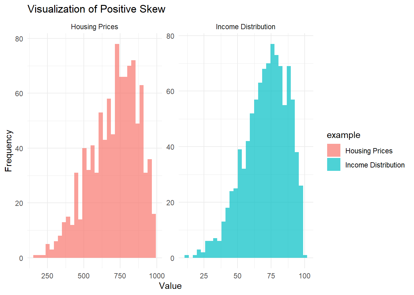
Figure 2.1: Visualization of positie skew
- In the Income Distribution example, most people earn moderate incomes, but a few high earners stretch the right tail.
- In the Housing Prices example, most homes are reasonably priced, but a few mansions create a long, expensive right tail.
- Negative Skew (Left Skew)
Negative skew occurs when the left tail (lower values) of the distribution is longer or heavier.
-
Examples:
Scores on an Easy Test: If an exam is very easy, most students score quite high, and only a few students score low, creating a left tail.
Age of Retirement: Most people might retire around a common age (say 65+), with fewer retiring very early (stretching the left tail).
# Simulate data for negative skew
set.seed(123)
negative_skew_test <-
    10 - rbeta(1000, 5, 2) * 10  # Easy test scores example
negative_skew_retirement <-
    80 - rbeta(1000, 5, 2) * 20  # Retirement age example

# Combine data
data_negative_skew <- data.frame(
    value = c(negative_skew_test, negative_skew_retirement),
    example = c(rep("Easy Test Scores", 1000),
                rep("Retirement Age", 1000))
)

# Plot negative skew
ggplot(data_negative_skew, aes(x = value, fill = example)) +
    geom_histogram(bins = 30,
                   alpha = 0.7,
                   position = "identity") +
    facet_wrap( ~ example, scales = "free") +
    labs(title = "Visualization of Negative Skew",
         x = "Value",
         y = "Frequency") +
    theme_minimal()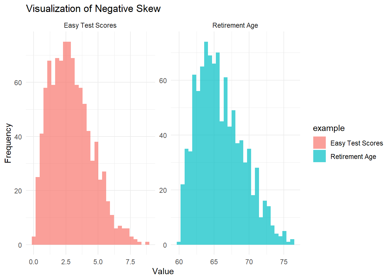
Figure 2.2: Visualization of negative skew
In the Easy Test Scores example, most students perform well, but a few low scores stretch the left tail.
In the Retirement Age example, most people retire around the same age, but a small number of individuals retire very early, stretching the left tail.
2.2.7 Kurtosis
Kurtosis measures the “peakedness” or heaviness of the tails:
-
High kurtosis: Tall, sharp peak with heavy tails.
- Example: Financial market returns during a crisis (extreme losses or gains).
-
Low kurtosis: Flatter peak with thinner tails.
- Example: Human height distribution (fewer extreme deviations from the mean).
# Simulate data for kurtosis
low_kurtosis <- runif(1000, 0, 10)
high_kurtosis <- c(rnorm(900, 5, 1), rnorm(100, 5, 5))

# Combine data
data_kurtosis <- data.frame(
  value = c(low_kurtosis, high_kurtosis),
  kurtosis_type = c(rep("Low Kurtosis (Height Distribution)", 1000),
                    rep("High Kurtosis (Market Returns)", 1000))
)

# Plot kurtosis
ggplot(data_kurtosis, aes(x = value, fill = kurtosis_type)) +
  geom_histogram(bins = 30, alpha = 0.7, position = "identity") +
  facet_wrap(~kurtosis_type) +
  labs(
    title = "Visualization of Kurtosis",
    x = "Value",
    y = "Frequency"
  ) +
  theme_minimal()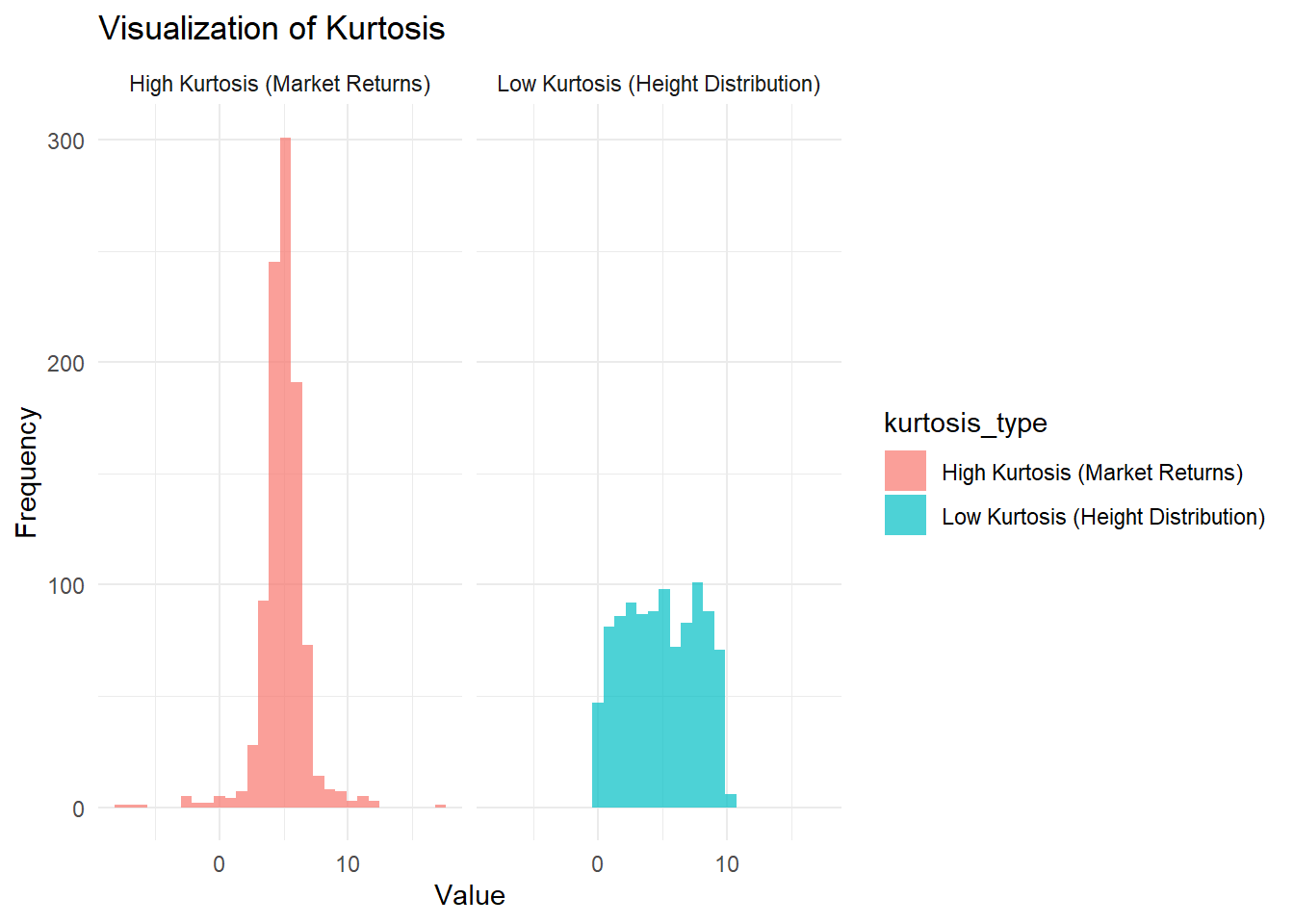
Figure 2.3: Visualization of kurtosis
The left panel shows low kurtosis, similar to the distribution of human height, which has a flatter peak and thinner tails.
The right panel shows high kurtosis, reflecting financial market returns, where there are more extreme outliers in gains or losses.
2.2.7.1 Conditional Moments
For a random variable \(Y\) given \(X=x\):
Expected Value: \[ E[Y|X=x] = \begin{cases} \sum_y y f_Y(y|x) & \text{for discrete RV}, \\ \int_y y f_Y(y|x) dy & \text{for continuous RV}. \end{cases} \]
Variance: \[ \text{Var}(Y|X=x) = \begin{cases} \sum_y (y - E[Y|X=x])^2 f_Y(y|x) & \text{for discrete RV}, \\ \int_y (y - E[Y|X=x])^2 f_Y(y|x) dy & \text{for continuous RV}. \end{cases} \]
2.2.7.2 Multivariate Moments
Expected Value: \[ E \begin{bmatrix} X \\ Y \end{bmatrix} = \begin{bmatrix} E[X] \\ E[Y] \end{bmatrix} = \begin{bmatrix} \mu_X \\ \mu_Y \end{bmatrix} \]
Variance-Covariance Matrix: \[ \begin{aligned} \text{Var} \begin{bmatrix} X \\ Y \end{bmatrix} &= \begin{bmatrix} \text{Var}(X) & \text{Cov}(X, Y) \\ \text{Cov}(X, Y) & \text{Var}(Y) \end{bmatrix} \\ &= \begin{bmatrix} E[(X-\mu_X)^2] & E[(X-\mu_X)(Y-\mu_Y)] \\ E[(X-\mu_X)(Y-\mu_Y)] & E[(Y-\mu_Y)^2] \end{bmatrix} \end{aligned} \]
2.2.7.3 Properties of Moments
- \(E[aX + bY + c] = aE[X] + bE[Y] + c\)
- \(\text{Var}(aX + bY + c) = a^2 \text{Var}(X) + b^2 \text{Var}(Y) + 2ab \text{Cov}(X, Y)\)
- \(\text{Cov}(aX + bY, cX + dY) = ac \text{Var}(X) + bd \text{Var}(Y) + (ad + bc) \text{Cov}(X, Y)\)
- Correlation: \(\rho_{XY} = \frac{\text{Cov}(X, Y)}{\sigma_X \sigma_Y}\)
2.2.8 Distributions
2.2.8.1 Conditional Distributions
\[ f_{X|Y}(x|y) = \frac{f(x, y)}{f_Y(y)} \]
If \(X\) and \(Y\) are independent:
\[ f_{X|Y}(x|y) = f_X(x). \]
2.2.8.2 Discrete Distributions
2.2.8.2.1 Bernoulli Distribution
A random variable \(X\) follows a Bernoulli distribution, denoted as \(X \sim \text{Bernoulli}(p)\), if it represents a single trial with:
Success probability \(p\)
Failure probability \(q = 1-p\).
Density Function\[ f(x) = p^x (1-p)^{1-x}, \quad x \in \{0, 1\} \]
CDF: Use table or manual computation.
hist(
    mc2d::rbern(1000, prob = 0.5),
    main = "Histogram of Bernoulli Distribution",
    xlab = "Value",
    ylab = "Frequency"
)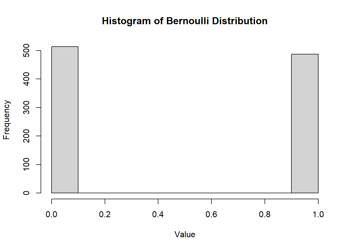
Figure 2.4: Histogram of Bernoulli Distribution
Mean
\[ \mu = E[X] = p \]
Variance
\[ \sigma^2 = \text{Var}(X) = p(1-p) \]
2.2.8.2.2 Binomial Distribution
\(X \sim B(n, p)\) is the number of successes in \(n\) independent Bernoulli trials, where:
\(n\) is the number of trials
\(p\) is the success probability.
The trials are identical and independent, and probability of success (\(p\)) and probability of failure (\(q = 1 - p\)) remains the same for all trials.
Density Function
\[ f(x) = \binom{n}{x} p^x (1-p)^{n-x}, \quad x = 0, 1, \dots, n \]
hist(
    rbinom(1000, size = 100, prob = 0.5),
    main = "Histogram of Binomial Distribution",
    xlab = "Value",
    ylab = "Frequency"
)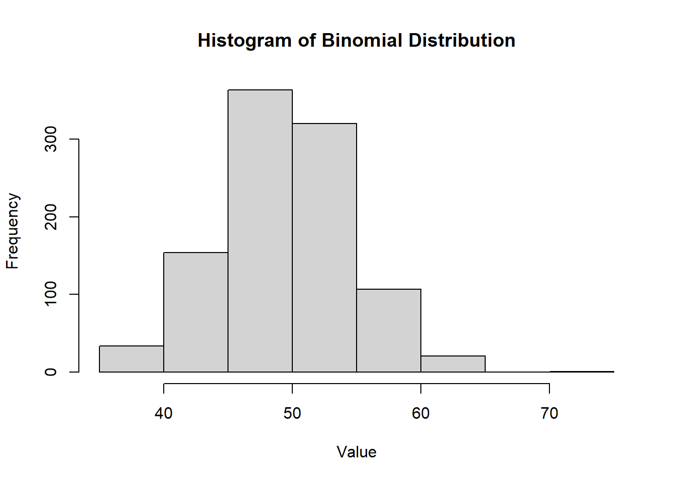
Figure 2.5: Histogram of Binomial Distribution
MGF
\[ m_X(t) = (1 - p + p e^t)^n \]
Mean
\[ \mu = np \]
Variance
\[ \sigma^2 = np(1-p) \]
2.2.8.2.3 Poisson Distribution
\(X \sim \text{Poisson}(\lambda)\) models the number of occurrences of an event in a fixed interval, with average rate \(\lambda\).
Arises with Poisson process, which involves observing discrete events in a continuous “interval” of time, length, or space.
The random variable \(X\) is the number of occurrences of the event within an interval of \(s\) units.
The parameter \(\lambda\) is the average number of occurrences of the event in question per measurement unit. For the distribution, we use the parameter \(k = \lambda s\).
Density Function
\[ f(x) = \frac{e^{-k} k^x}{x!}, \quad x = 0, 1, 2, \dots \]
CDF
hist(rpois(1000, lambda = 5),
     main = "Histogram of Poisson Distribution",
     xlab = "Value",
     ylab = "Frequency")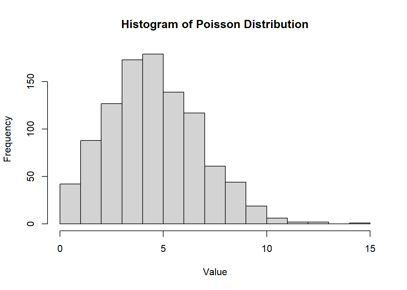
Figure 2.6: Histogram of Poisson Distribution
MGF
\[ m_X(t) = e^{k (e^t - 1)} \]
Mean
\[ \mu = E(X) = k \]
Variance
\[ \sigma^2 = Var(X) = k \]
2.2.8.2.4 Geometric Distribution
\(X \sim \text{G}(p)\) models the number of trials needed to obtain the first success, with:
\(p\): probability of success
\(q = 1-p\): probability of failure.
The experiment consists of a series of trails. The outcome of each trial can be classed as being either a “success” (s) or “failure” (f). (i.e., Bernoulli trial).
The trials are identical and independent in the sense that the outcome of one trial has no effect on the outcome of any other (i..e, lack of memory - momerylessness). The probability of success (\(p\)) and probability of failure (\(q = 1- p\)) remains the same from trial to trial.
Density Function
\[ f(x) = p(1-p)^{x-1}, \quad x = 1, 2, \dots \]
CDF\[ F(x) = 1 - (1-p)^x \]
hist(rgeom(1000, prob = 0.5),
     main = "Histogram of Geometric Distribution",
     xlab = "Value",
     ylab = "Frequency")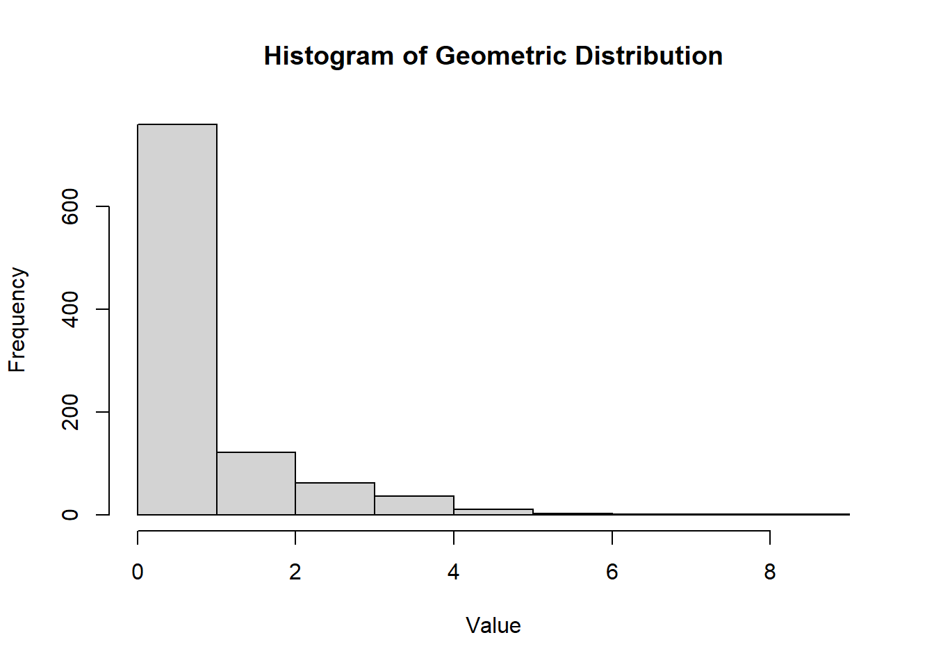
Figure 2.7: Histogram of Geometric Distribution
MGF
\[ m_X(t) = \frac{p e^t}{1 - (1-p)e^t}, \quad t < -\ln(1-p) \]
Mean
\[ \mu = \frac{1}{p} \]
Variance
\[ \sigma^2 = \frac{1-p}{p^2} \]
2.2.8.2.5 Hypergeometric Distribution
\(X \sim \text{H}(N, r, n)\) models the number of successes in a sample of size \(n\) drawn without replacement from a population of size \(N\), where:
\(r\) objects have the trait of interest
\(N-r\) do not have the trait.
Density Function
\[ f(x) = \frac{\binom{r}{x} \binom{N-r}{n-x}}{\binom{N}{n}}, \quad \max(0, n-(N-r)) \leq x \leq \min(n, r) \]
hist(
    rhyper(1000, m = 50, n = 20, k = 30),
    main = "Histogram of Hypergeometric Distribution",
    xlab = "Value",
    ylab = "Frequency"
)
Figure 2.8: Histogram of Hypergeometric Distribution
Mean\[ \mu = E[X] = \frac{n r}{N} \]
Variance\[ \sigma^2 = \text{Var}(X) = n \frac{r}{N} \frac{N-r}{N} \frac{N-n}{N-1} \]
Note: For large \(N\) (when \(\frac{n}{N} \leq 0.05\)), the hypergeometric distribution can be approximated by a binomial distribution with \(p = \frac{r}{N}\).
2.2.8.3 Continuous Distributions
2.2.8.3.1 Uniform Distribution
Defined over an interval \((a, b)\), where the probabilities are “equally likely” for subintervals of equal length.
Density Function: \[ f(x) = \frac{1}{b-a}, \quad a < x < b \]
CDF\[ F(x) = \begin{cases} 0 & \text{if } x < a \\ \frac{x-a}{b-a} & a \le x \le b \\ 1 & \text{if } x > b \end{cases} \]
hist(
    runif(1000, min = 0, max = 1),
    main = "Histogram of Uniform Distribution",
    xlab = "Value",
    ylab = "Frequency"
)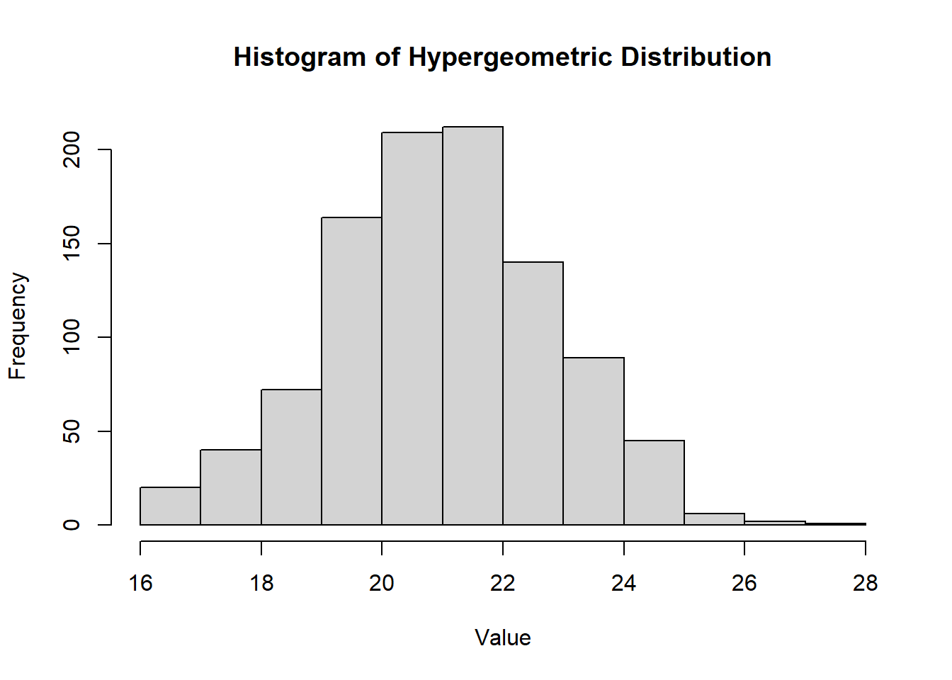
Figure 2.9: Histogram of Uniform Distribution
MGF\[ m_X(t) = \begin{cases} \frac{e^{tb} - e^{ta}}{t(b-a)} & \text{if } t \neq 0 \\ 1 & \text{if } t = 0 \end{cases} \]
Mean\[ \mu = E[X] = \frac{a + b}{2} \]
Variance
\[ \sigma^2 = \text{Var}(X) = \frac{(b-a)^2}{12} \]
2.2.8.3.2 Gamma Distribution
The gamma distribution is used to define the exponential and \(\chi^2\) distributions.
The gamma function is defined as: \[ \Gamma(\alpha) = \int_0^{\infty} z^{\alpha-1}e^{-z}dz, \quad \alpha > 0 \]
Properties of the Gamma Function:
\(\Gamma(1) = 1\)
For \(\alpha > 1\), \(\Gamma(\alpha) = (\alpha-1)\Gamma(\alpha-1)\)
If \(n\) is an integer and \(n > 1\), then \(\Gamma(n) = (n-1)!\)
Density Function:
\[ f(x) = \frac{1}{\Gamma(\alpha)\beta^{\alpha}} x^{\alpha-1} e^{-x/\beta}, \quad x > 0 \]
CDF (for \(\alpha = n\), and \(x>0\) a positive integer):
\[ F(x, n, \beta) = 1 - \sum_{k=0}^{n-1} \frac{(\frac{x}{\beta})^k e^{-x/\beta}}{k!} \]
PDF:
hist(
    rgamma(n = 1000, shape = 5, rate = 1),
    main = "Histogram of Gamma Distribution",
    xlab = "Value",
    ylab = "Frequency"
)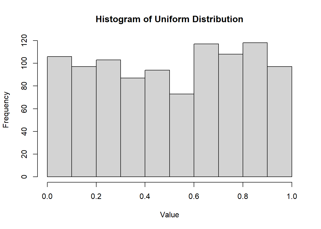
Figure 2.10: Histogram of Gamma Distribution
MGF
\[ m_X(t) = (1 - \beta t)^{-\alpha}, \quad t < \frac{1}{\beta} \]
Mean
\[ \mu = E[X] = \alpha \beta \]
Variance
\[ \sigma^2 = \text{Var}(X) = \alpha \beta^2 \]
2.2.8.3.3 Normal Distribution
The normal distribution, denoted as \(N(\mu, \sigma^2)\), is symmetric and bell-shaped with parameters \(\mu\) (mean) and \(\sigma^2\) (variance). It is also known as the Gaussian distribution.
Density Function:
\[ f(x) = \frac{1}{\sigma \sqrt{2\pi}} e^{-\frac{1}{2} \left(\frac{x-\mu}{\sigma}\right)^2}, \quad -\infty < x < \infty, \sigma > 0 \]
CDF: Use table or numerical methods.
hist(
    rnorm(1000, mean = 0, sd = 1),
    main = "Histogram of Normal Distribution",
    xlab = "Value",
    ylab = "Frequency"
)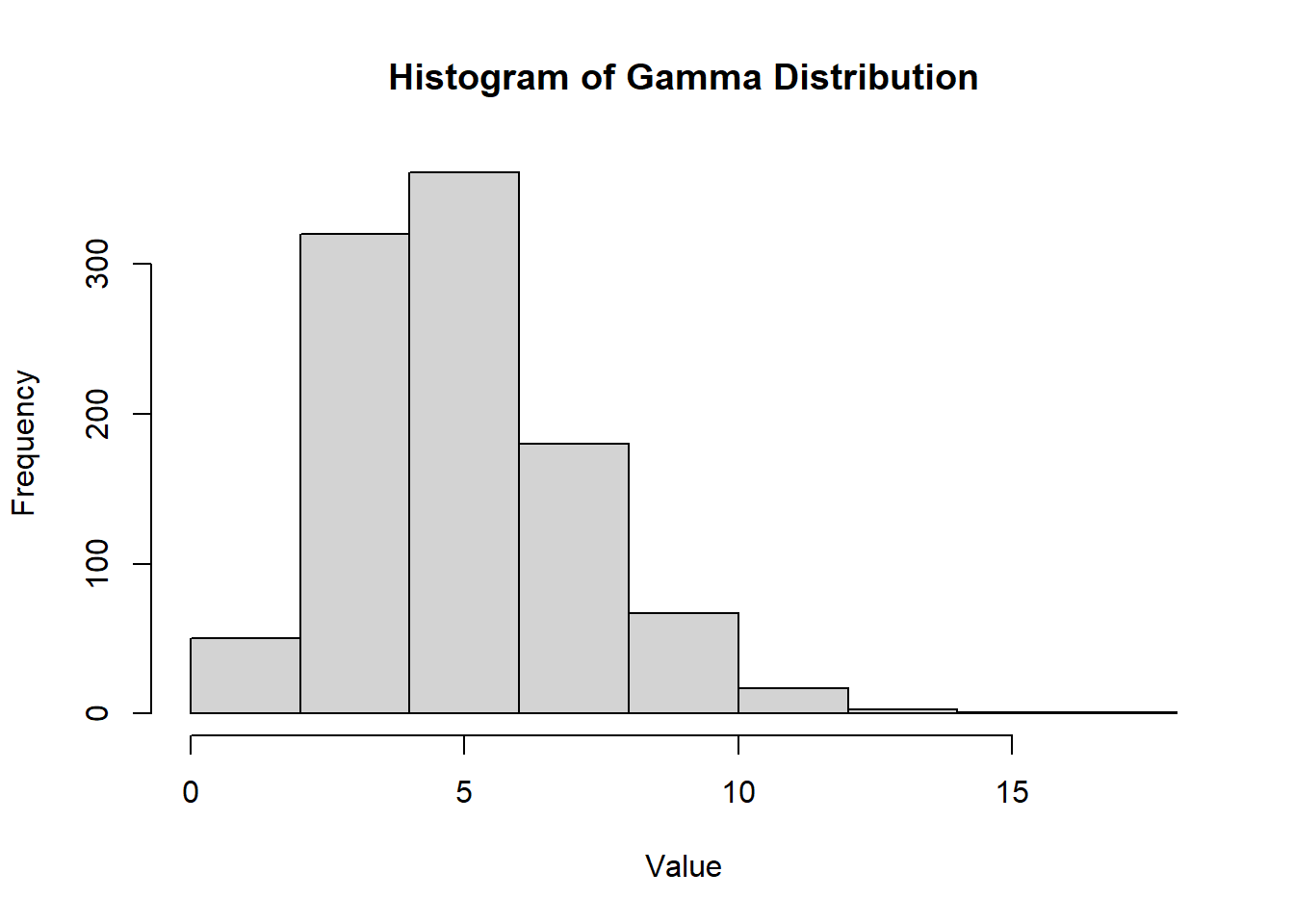
Figure 2.11: Histogram of Normal Distribution
MGF
\[ m_X(t) = e^{\mu t + \frac{\sigma^2 t^2}{2}} \]
Mean
\[ \mu = E[X] \]
Variance
\[ \sigma^2 = \text{Var}(X) \]
Standard Normal Random Variable:
The normal random variable \(Z\) with mean \(\mu = 0\) and standard deviation \(\sigma = 1\) is called a standard normal random variable.
Any normal random variable \(X\) with mean \(\mu\) and standard deviation \(\sigma\) can be converted to the standard normal random variable \(Z\): \[ Z = \frac{X - \mu}{\sigma} \]
Normal Approximation to the Binomial Distribution:
Let \(X\) be binomial with parameters \(n\) and \(p\). For large \(n\):
If \(p \le 0.5\) and \(np > 5\), or
If \(p > 0.5\) and \(n(1-p) > 5\),
\(X\) is approximately normally distributed with mean \(\mu = np\) and standard deviation \(\sigma = \sqrt{np(1-p)}\).
When using the normal approximation, add or subtract 0.5 as needed for the continuity correction.
Discrete Approximate Normal (Corrected):
| Discrete | Approximate Normal (corrected) |
|---|---|
| \(P(X = c)\) | \(P(c -0.5 < Y < c + 0.5)\) |
| \(P(X < c)\) | \(P(Y < c - 0.5)\) |
| \(P(X \le c)\) | \(P(Y < c + 0.5)\) |
| \(P(X > c)\) | \(P(Y > c + 0.5)\) |
| \(P(X \ge c)\) | \(P(Y > c - 0.5)\) |
Normal Probability Rule
If X is normally distributed with parameters \(\mu\) and \(\sigma\), then
- \(P(-\sigma < X - \mu < \sigma) \approx .68\)
- \(P(-2\sigma < X - \mu < 2\sigma) \approx .95\)
- \(P(-3\sigma < X - \mu < 3\sigma) \approx .997\)
2.2.8.3.4 Logistic Distribution
The logistic distribution is a continuous probability distribution commonly used in logistic regression and other types of statistical modeling. It resembles the normal distribution but has heavier tails, allowing for more extreme values. - The logistic distribution is symmetric around \(\mu\). - Its heavier tails make it useful for modeling outcomes with occasional extreme values.
Density Function
\[ f(x; \mu, s) = \frac{e^{-(x-\mu)/s}}{s \left(1 + e^{-(x-\mu)/s}\right)^2}, \quad -\infty < x < \infty \]
where \(\mu\) is the location parameter (mean) and \(s > 0\) is the scale parameter.
CDF
\[ F(x; \mu, s) = \frac{1}{1 + e^{-(x-\mu)/s}}, \quad -\infty < x < \infty \]
hist(
    rlogis(1000, location = 0, scale = 1),
    main = "Histogram of Logistic Distribution",
    xlab = "Value",
    ylab = "Frequency"
)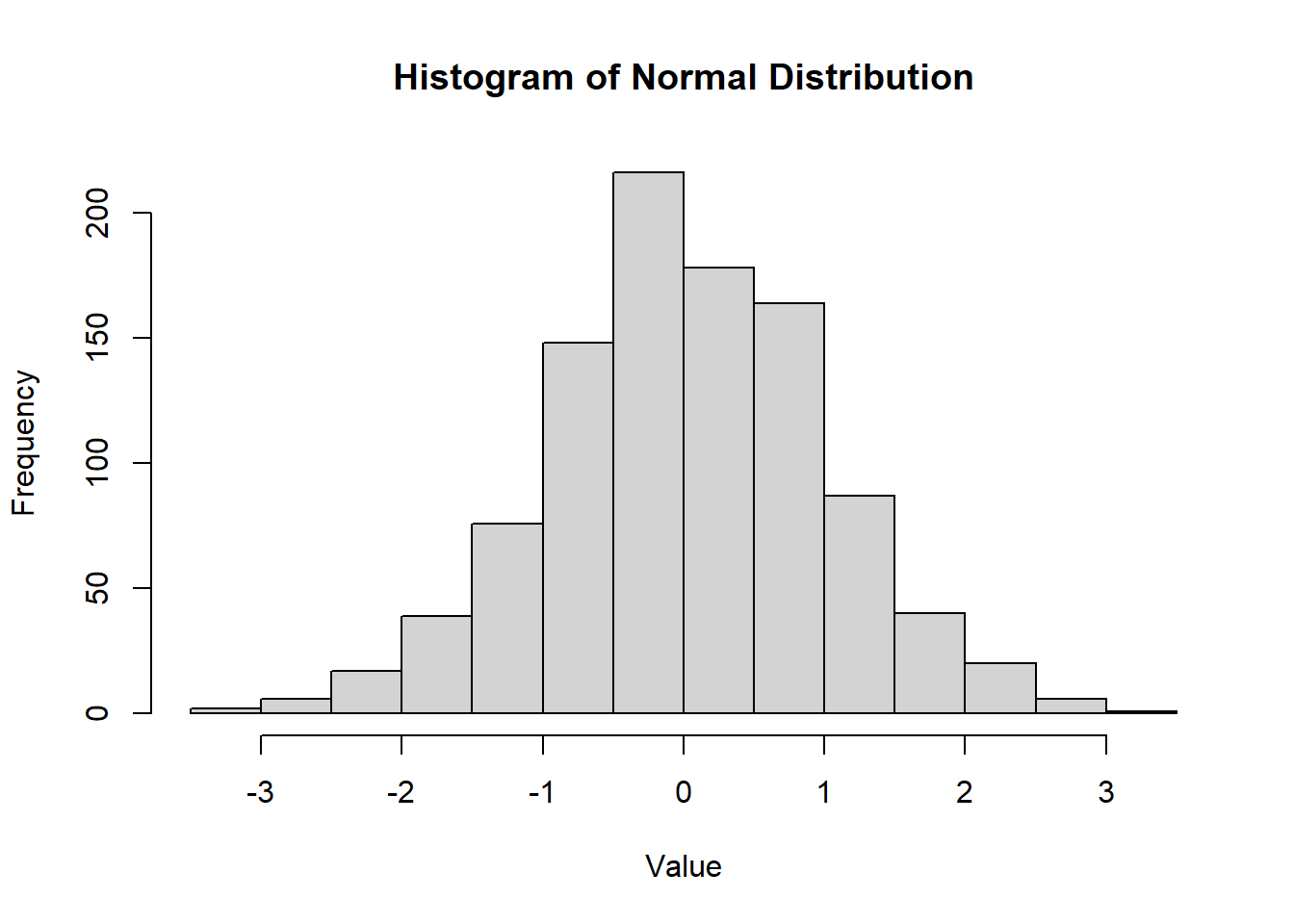
Figure 2.12: Histogram of Logistic Distribution
MGF
The MGF of the logistic distribution does not exist because its expected value diverges for most \(t\).
Mean
\[ \mu = E[X] = \mu \]
Variance
\[ \sigma^2 = \text{Var}(X) = \frac{\pi^2 s^2}{3} \]
2.2.8.3.5 Laplace Distribution
The Laplace distribution, also known as the double exponential distribution, is a continuous probability distribution often used in economics, finance, and engineering. It is characterized by a peak at its mean and heavier tails compared to the normal distribution.
- The Laplace distribution is symmetric around \(\mu\).
- It has heavier tails than the normal distribution, making it suitable for modeling data with more extreme outliers.
Density Function
\[ f(x; \mu, b) = \frac{1}{2b} e^{-|x-\mu|/b}, \quad -\infty < x < \infty \]
where \(\mu\) is the location parameter (mean) and \(b > 0\) is the scale parameter.
CDF
\[ F(x; \mu, b) = \begin{cases} \frac{1}{2} e^{(x-\mu)/b} & \text{if } x < \mu \\ 1 - \frac{1}{2} e^{-(x-\mu)/b} & \text{if } x \ge \mu \end{cases} \]
hist(
    VGAM::rlaplace(1000, location = 0, scale = 1),
    main = "Histogram of Laplace Distribution",
    xlab = "Value",
    ylab = "Frequency"
)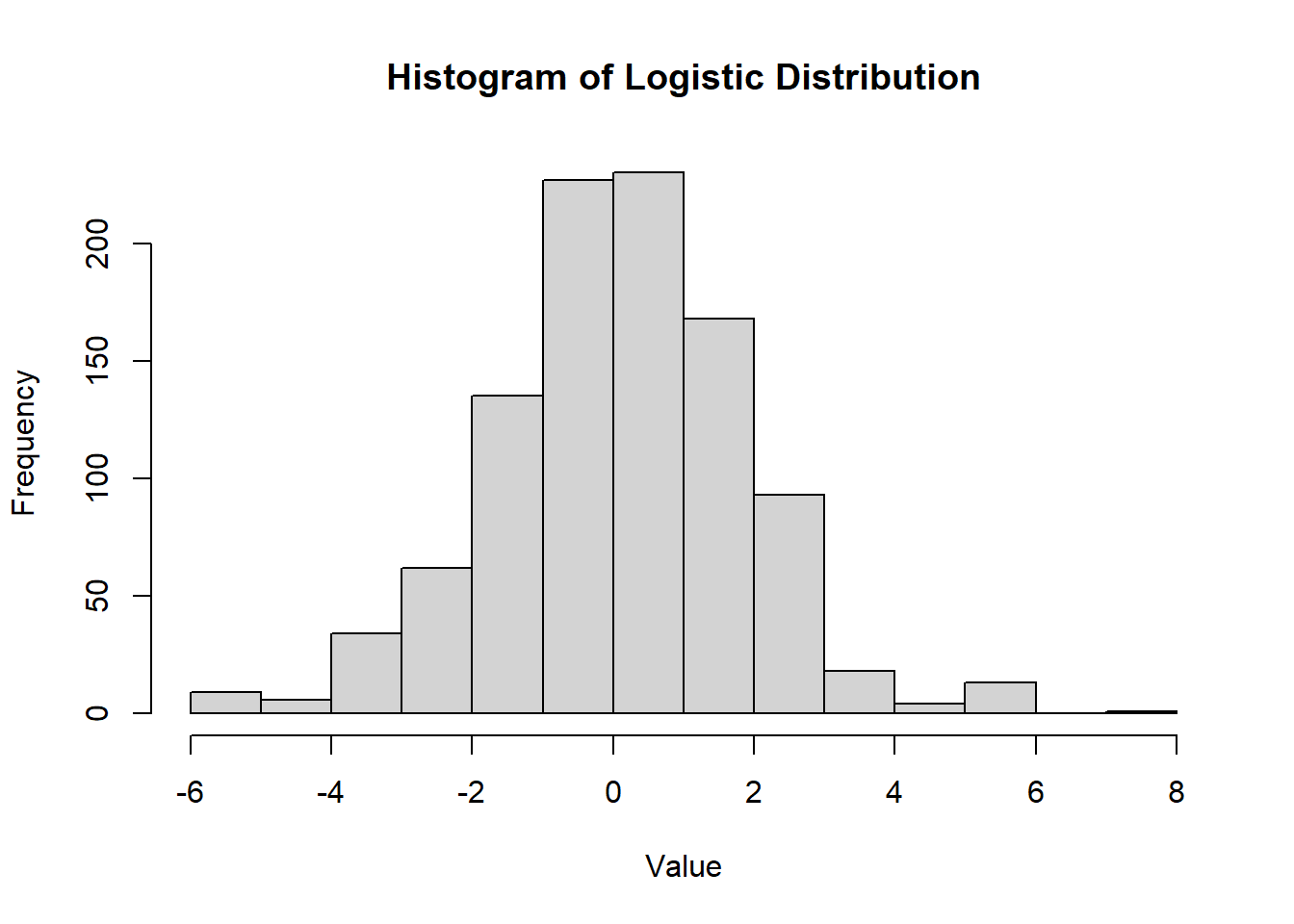
Figure 2.13: Histogram of Laplace Distribution
MGF
\[ m_X(t) = \frac{e^{\mu t}}{1 - b^2 t^2}, \quad |t| < \frac{1}{b} \]
Mean
\[ \mu = E[X] = \mu \]
Variance
\[ \sigma^2 = \text{Var}(X) = 2b^2 \]
2.2.8.3.6 Lognormal Distribution
The lognormal distribution is a continuous probability distribution of a random variable whose logarithm is normally distributed. It is often used to model variables that are positively skewed, such as income or biological measurements.
- The lognormal distribution is positively skewed.
- It is useful for modeling data that cannot take negative values and is often used in finance and environmental studies.
Density Function
\[ f(x; \mu, \sigma) = \frac{1}{x \sigma \sqrt{2\pi}} e^{-(\ln(x) - \mu)^2 / (2\sigma^2)}, \quad x > 0 \]
where \(\mu\) is the mean of the underlying normal distribution and \(\sigma > 0\) is the standard deviation.
CDF
The cumulative distribution function of the lognormal distribution is given by:
\[ F(x; \mu, \sigma) = \frac{1}{2} \left[ 1 + \text{erf}\left( \frac{\ln(x) - \mu}{\sigma \sqrt{2}} \right) \right], \quad x > 0 \]
hist(
    rlnorm(1000, meanlog = 0, sdlog = 1),
    main = "Histogram of Lognormal Distribution",
    xlab = "Value",
    ylab = "Frequency"
)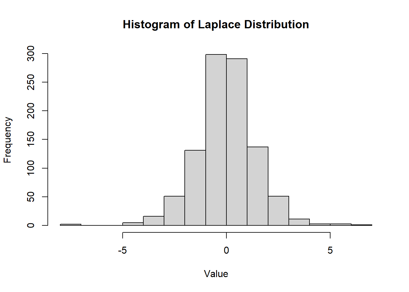
Figure 2.14: Histogram of Lognormal Distribution
MGF
The moment generating function (MGF) of the lognormal distribution does not exist in a simple closed form.
Mean
\[ E[X] = e^{\mu + \sigma^2 / 2} \]
Variance
\[ \sigma^2 = \text{Var}(X) = \left( e^{\sigma^2} - 1 \right) e^{2\mu + \sigma^2} \]
2.2.8.3.7 Exponential Distribution
The exponential distribution, denoted as \(\text{Exp}(\lambda)\), is a special case of the gamma distribution with \(\alpha = 1\).
It is commonly used to model the time between independent events that occur at a constant rate. It is often applied in reliability analysis and queuing theory.
The exponential distribution is memoryless, meaning the probability of an event occurring in the future is independent of the past.
It is commonly used to model waiting times, such as the time until the next customer arrives or the time until a radioactive particle decays.
Density Function
\[ f(x) = \frac{1}{\beta} e^{-x/\beta}, \quad x, \beta > 0 \]
CDF\[ F(x) = \begin{cases} 0 & \text{if } x \le 0 \\ 1 - e^{-x/\beta} & \text{if } x > 0 \end{cases} \]
hist(rexp(n = 1000, rate = 1),
     main = "Histogram of Exponential Distribution",
     xlab = "Value",
     ylab = "Frequency")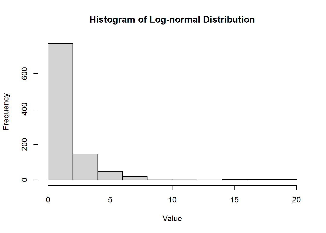
Figure 2.15: Histogram of Exponential Distribution
MGF\[ m_X(t) = (1-\beta t)^{-1}, \quad t < 1/\beta \]
Mean\[ \mu = E[X] = \beta \]
Variance\[ \sigma^2 = \text{Var}(X) = \beta^2 \]
2.2.8.3.8 Chi-Squared Distribution
The chi-squared distribution is a continuous probability distribution commonly used in statistical inference, particularly in hypothesis testing and construction of confidence intervals for variance. It is also used in goodness-of-fit tests.
- The chi-squared distribution is defined only for positive values.
- It is often used to model the distribution of the sum of the squares of \(k\) independent standard normal random variables.
Density Function
\[ f(x; k) = \frac{1}{2^{k/2} \Gamma(k/2)} x^{k/2 - 1} e^{-x/2}, \quad x \ge 0 \]
where \(k\) is the degrees of freedom and \(\Gamma\) is the gamma function.
CDF
The cumulative distribution function of the chi-squared distribution is given by:
\[ F(x; k) = \frac{\gamma(k/2, x/2)}{\Gamma(k/2)}, \quad x \ge 0 \]
where \(\gamma\) is the lower incomplete gamma function.
hist(
    rchisq(1000, df = 5),
    main = "Histogram of Chi-Squared Distribution",
    xlab = "Value",
    ylab = "Frequency"
)
Figure 2.16: Histogram of Chi-Squared Distribution
MGF
\[ m_X(t) = (1 - 2t)^{-k/2}, \quad t < \frac{1}{2} \]
Mean
\[ E[X] = k \]
Variance
\[ \sigma^2 = \text{Var}(X) = 2k \]
2.2.8.3.9 Student’s T Distribution
The Student’s t-distribution is named after William Sealy Gosset, a statistician at Guinness Brewery in the early 20th century. Gosset developed the t-distribution to address small-sample problems in quality control. Since Guinness prohibited employees from publishing under their names, Gosset used the pseudonym “Student” when he published his work in 1908 (Student 1908). The name has stuck ever since, honoring his contribution to statistics.
The Student’s t-distribution, denoted as \(T(v)\), is defined by: \[ T = \frac{Z}{\sqrt{\chi^2_v / v}}, \] where \(Z\) is a standard normal random variable and \(\chi^2_v\) follows a chi-squared distribution with \(v\) degrees of freedom.
The Student’s T distribution is a continuous probability distribution used in statistical inference, particularly for estimating population parameters when the sample size is small and/or the population variance is unknown. It is similar to the normal distribution but has heavier tails, which makes it more robust for small sample sizes.
- The Student’s T distribution is symmetric around 0.
- It has heavier tails than the normal distribution, making it useful for dealing with outliers or small sample sizes.
Density Function
\[ f(x;v) = \frac{\Gamma((v + 1)/2)}{\sqrt{v \pi} \Gamma(v/2)} \left( 1 + \frac{x^2}{v} \right)^{-(v + 1)/2} \]
where \(v\) is the degrees of freedom and \(\Gamma(x)\) is the Gamma function.
CDF
The cumulative distribution function of the Student’s T distribution is more complex and typically evaluated using numerical methods.
hist(
    rt(1000, df = 5),
    main = "Histogram of Student's T Distribution",
    xlab = "Value",
    ylab = "Frequency"
)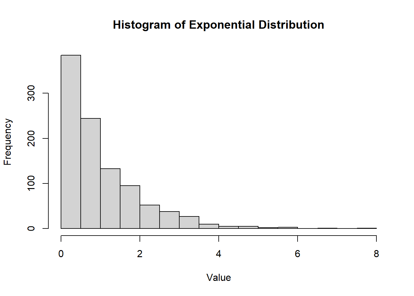
Figure 2.17: Histogram of Student’s T Distribution.
MGF
The moment generating function (MGF) of the Student’s T distribution does not exist in a simple closed form.
Mean
For \(v > 1\):
\[ E[X] = 0 \]
Variance
For \(v > 2\):
\[ \sigma^2 = \text{Var}(X) = \frac{v}{v - 2} \]
2.2.8.3.10 Non-central T Distribution
The non-central t-distribution, denoted as \(T(v, \lambda)\), is a generalization of the Student’s t-distribution. It is defined as: \[ T = \frac{Z + \lambda}{\sqrt{\chi^2_v / v}}, \] where \(Z\) is a standard normal random variable, \(\chi^2_v\) follows a chi-squared distribution with \(v\) degrees of freedom, and \(\lambda\) is the non-centrality parameter. This additional parameter introduces asymmetry to the distribution.
The non-central t-distribution arises in scenarios where the null hypothesis does not hold, such as under the alternative hypothesis in hypothesis testing. The non-centrality parameter \(\lambda\) represents the degree to which the mean deviates from zero.
- For \(\lambda = 0\), the non-central t-distribution reduces to the Student’s t-distribution.
- The distribution is skewed for \(\lambda \neq 0\), with the skewness increasing as \(\lambda\) grows.
Density Function
The density function of the non-central t-distribution is more complex and depends on \(v\) and \(\lambda\). It can be expressed in terms of an infinite sum:
\[ f(x; v, \lambda) = \sum_{k=0}^\infty \frac{e^{-\lambda^2/2}(\lambda^2/2)^k}{k!} \cdot \frac{\Gamma((v + k + 1)/2)}{\sqrt{v \pi} \Gamma((v + k)/2)} \left( 1 + \frac{x^2}{v} \right)^{-(v + k + 1)/2}. \]
n <- 100  # Number of samples
df <- 5    # Degrees of freedom
lambda <- 2  # Non-centrality parameter


hist(
  rt(n, df = df, ncp = lambda),
  main = "Histogram of Non-central T Distribution",
  xlab = "Value",
  ylab = "Frequency"
)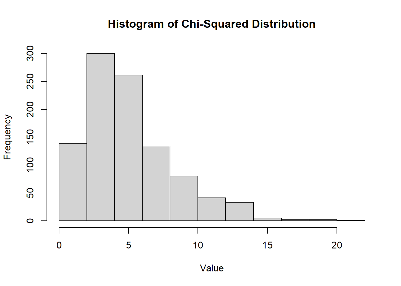
Figure 2.18: Histogram of Non-central T Distribution
CDF
The cumulative distribution function of the non-central t-distribution is typically computed using numerical methods due to its complexity.
Mean
For \(v > 1\):
\[ E[T] = \lambda \sqrt{\frac{v}{2}} \cdot \frac{\Gamma((v - 1)/2)}{\Gamma(v/2)}. \]
Variance
For \(v > 2\):
\[ \text{Var}(T) = \frac{v}{v - 2} + \lambda^2. \]
| Feature | Student’s t-distribution | Non-central t-distribution |
|---|---|---|
| Definition | \(T = \frac{Z}{\sqrt{\chi^2_v / v}}\) | \(T = \frac{Z + \lambda}{\sqrt{\chi^2_v / v}}\) |
| Centered at | 0 | \(\lambda\) |
| Symmetry | Symmetric | Skewed for \(\lambda \neq 0\) |
| Parameters | Degrees of freedom (\(v\)) | \(v\) and \(\lambda\) |
|
Shape as \(v \to \infty\) (df \(\to \infty\)) |
Normal(0, 1) | Normal(\(\lambda\), 1) |
| Applications | Hypothesis testing under null | Power analysis, alternative testing |
While the Student’s \(t\)-distribution is used for standard hypothesis testing and confidence intervals, the non-central t-distribution finds its applications in scenarios involving non-null hypotheses, such as power and sample size calculations.
2.2.8.3.11 F Distribution
The F-distribution, denoted as \(F(d_1, d_2)\), is strictly positive and used to compare variances.
Definition: \[ F = \frac{\chi^2_{d_1} / d_1}{\chi^2_{d_2} / d_2}, \] where \(\chi^2_{d_1}\) and \(\chi^2_{d_2}\) are independent chi-squared random variables with degrees of freedom \(d_1\) and \(d_2\), respectively.
The distribution is asymmetric and never negative.
The F distribution arises frequently as the null distribution of a test statistic, especially in the context of comparing variances, such as in analysis of variance (ANOVA).
Density Function
\[ f(x; d_1, d_2) = \frac{\sqrt{\frac{(d_1 x)^{d_1} d_2^{d_2}}{(d_1 x + d_2)^{d_1 + d_2}}}}{x B\left( \frac{d_1}{2}, \frac{d_2}{2} \right)}, \quad x > 0 \]
where \(d_1\) and \(d_2\) are the degrees of freedom and \(B\) is the beta function.
CDF
The cumulative distribution function of the F distribution is typically evaluated using numerical methods.
hist(
    rf(1000, df1 = 5, df2 = 2),
    main = "Histogram of F Distribution",
    xlab = "Value",
    ylab = "Frequency"
)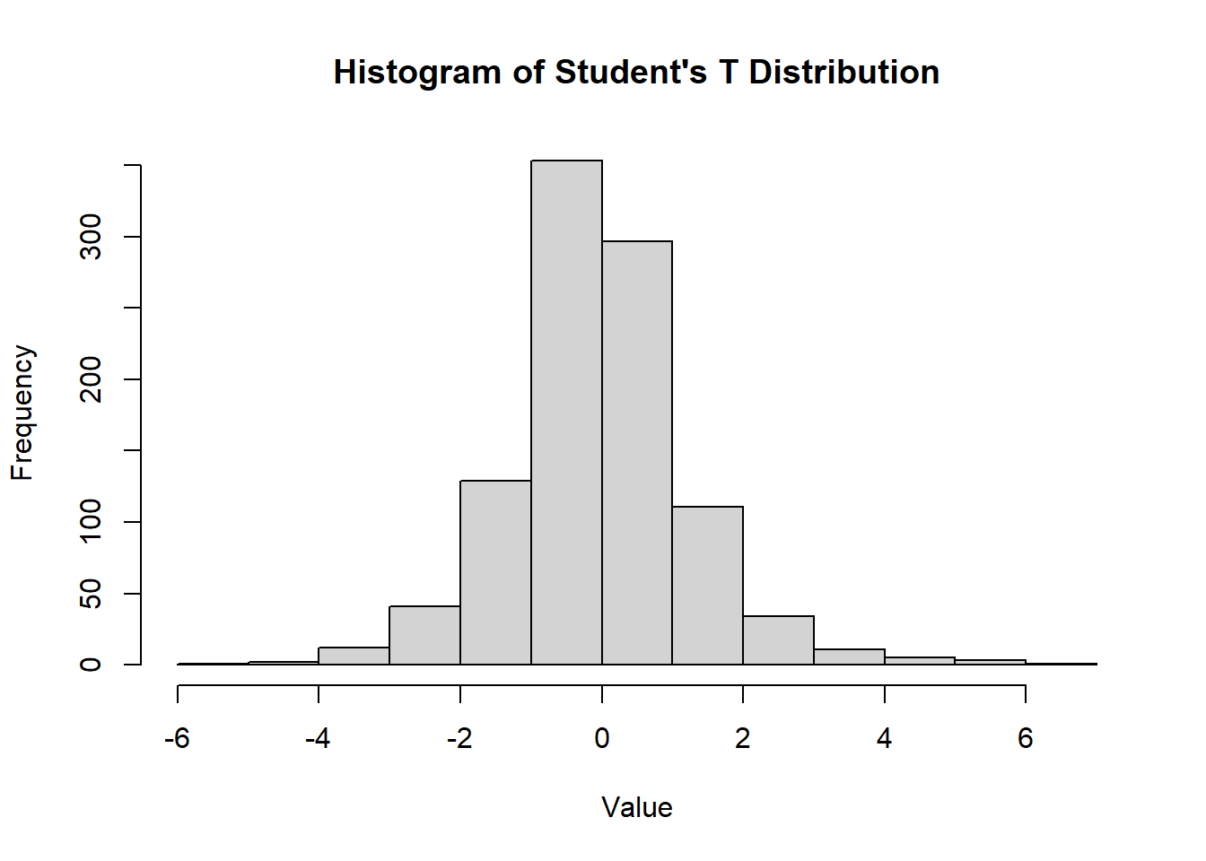
Figure 2.19: Histogram of F Distribution
MGF
The moment generating function (MGF) of the F distribution does not exist in a simple closed form.
Mean
For \(d_2 > 2\):
\[ E[X] = \frac{d_2}{d_2 - 2} \]
Variance
For \(d_2 > 4\):
\[ \sigma^2 = \text{Var}(X) = \frac{2 d_2^2 (d_1 + d_2 - 2)}{d_1 (d_2 - 2)^2 (d_2 - 4)} \]
2.2.8.3.12 Cauchy Distribution
The Cauchy distribution is a continuous probability distribution that is often used in physics and has heavier tails than the normal distribution. It is notable because it does not have a finite mean or variance.
- The Cauchy distribution does not have a finite mean or variance.
- The Central Limit Theorem and Weak Law of Large Numbers do not apply to the Cauchy distribution.
Density Function
\[ f(x; x_0, \gamma) = \frac{1}{\pi \gamma \left[ 1 + \left( \frac{x - x_0}{\gamma} \right)^2 \right]} \]
where \(x_0\) is the location parameter and \(\gamma > 0\) is the scale parameter.
CDF
The cumulative distribution function of the Cauchy distribution is given by:
\[ F(x; x_0, \gamma) = \frac{1}{\pi} \arctan \left( \frac{x - x_0}{\gamma} \right) + \frac{1}{2} \]
hist(
    rcauchy(1000, location = 0, scale = 1),
    main = "Histogram of Cauchy Distribution",
    xlab = "Value",
    ylab = "Frequency"
)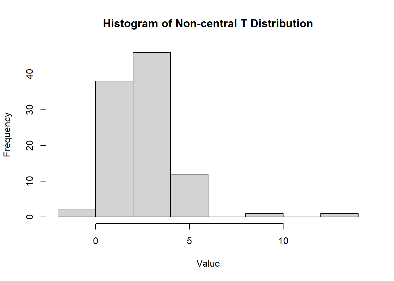
Figure 2.20: Histogram of Cauchy Distribution
MGF
The MGF of the Cauchy distribution does not exist.
Mean
The mean of the Cauchy distribution is undefined.
Variance
The variance of the Cauchy distribution is undefined.
2.2.8.3.13 Multivariate Normal Distribution
Let \(y\) be a \(p\)-dimensional multivariate normal (MVN) random variable with mean \(\mu\) and variance-covariance matrix \(\Sigma\). The density function of \(y\) is given by:
\[ f(\mathbf{y}) = \frac{1}{(2\pi)^{p/2}|\mathbf{\Sigma}|^{1/2}} \exp\left(-\frac{1}{2} (\mathbf{y}-\mu)' \Sigma^{-1} (\mathbf{y}-\mu)\right) \]
where \(|\mathbf{\Sigma}|\) represents the determinant of the variance-covariance matrix \(\Sigma\), and \(\mathbf{y} \sim N_p(\mathbf{\mu}, \mathbf{\Sigma})\).
Properties:
- Let \(\mathbf{A}_{r \times p}\) be a fixed matrix. Then \(\mathbf{A y} \sim N_r(\mathbf{A \mu}, \mathbf{A \Sigma A'})\). Note that \(r \le p\), and all rows of \(\mathbf{A}\) must be linearly independent to guarantee that \(\mathbf{A \Sigma A'}\) is non-singular.
- Let \(\mathbf{G}\) be a matrix such that \(\mathbf{\Sigma^{-1} = G G'}\). Then \(\mathbf{G'y} \sim N_p(\mathbf{G'\mu}, \mathbf{I})\) and \(\mathbf{G'(y - \mu)} \sim N_p(\mathbf{0}, \mathbf{I})\).
- Any fixed linear combination of \(y_1, \dots, y_p\), say \(\mathbf{c'y}\), follows \(\mathbf{c'y} \sim N_1(\mathbf{c'\mu}, \mathbf{c'\Sigma c})\).
Large Sample Properties
Suppose that \(y_1, \dots, y_n\) are a random sample from some population with mean \(\mu\) and variance-covariance matrix \(\Sigma\):
\[ \mathbf{Y} \sim MVN(\mathbf{\mu}, \mathbf{\Sigma}) \]
Then:
- \(\bar{\mathbf{y}} = \frac{1}{n} \sum_{i=1}^n \mathbf{y}_i\) is a consistent estimator for \(\mathbf{\mu}\).
- \(\mathbf{S} = \frac{1}{n-1} \sum_{i=1}^n (\mathbf{y}_i - \bar{\mathbf{y}})(\mathbf{y}_i - \bar{\mathbf{y}})'\) is a consistent estimator for \(\mathbf{\Sigma}\).
- Multivariate Central Limit Theorem: Similar to the univariate case, \(\sqrt{n}(\bar{\mathbf{y}} - \mu) \sim N_p(\mathbf{0}, \mathbf{\Sigma})\) when \(n\) is large relative to \(p\) (e.g., \(n \ge 25p\)), which is equivalent to \(\bar{\mathbf{y}} \sim N_p(\mathbf{\mu}, \mathbf{\Sigma/n})\).
- Wald’s Theorem: \(n(\bar{\mathbf{y}} - \mu)' \mathbf{S^{-1}} (\bar{\mathbf{y}} - \mu) \sim \chi^2_{(p)}\) when \(n\) is large relative to \(p\).
Density Function
\[ f(\mathbf{x}; \boldsymbol{\mu}, \boldsymbol{\Sigma}) = \frac{1}{(2\pi)^{k/2} | \boldsymbol{\Sigma}|^{1/2}} \exp\left( -\frac{1}{2} (\mathbf{x} - \boldsymbol{\mu})^T \boldsymbol{\Sigma}^{-1} (\mathbf{x} - \boldsymbol{\mu}) \right) \]
where \(\boldsymbol{\mu}\) is the mean vector, \(\boldsymbol{\Sigma}\) is the covariance matrix, \(\mathbf{x} \in \mathbb{R}^k\) and \(k\) is the number of variables.
CDF
The cumulative distribution function of the multivariate normal distribution does not have a simple closed form and is typically evaluated using numerical methods.
k <- 2
n <- 1000
mu <- c(0, 0)
sigma <- matrix(c(1, 0.5, 0.5, 1), nrow = k)
library(MASS)
hist(
    mvrnorm(n, mu = mu, Sigma = sigma)[,1],
    main = "Histogram of MVN Distribution (1st Var)",
    xlab = "Value",
    ylab = "Frequency"
)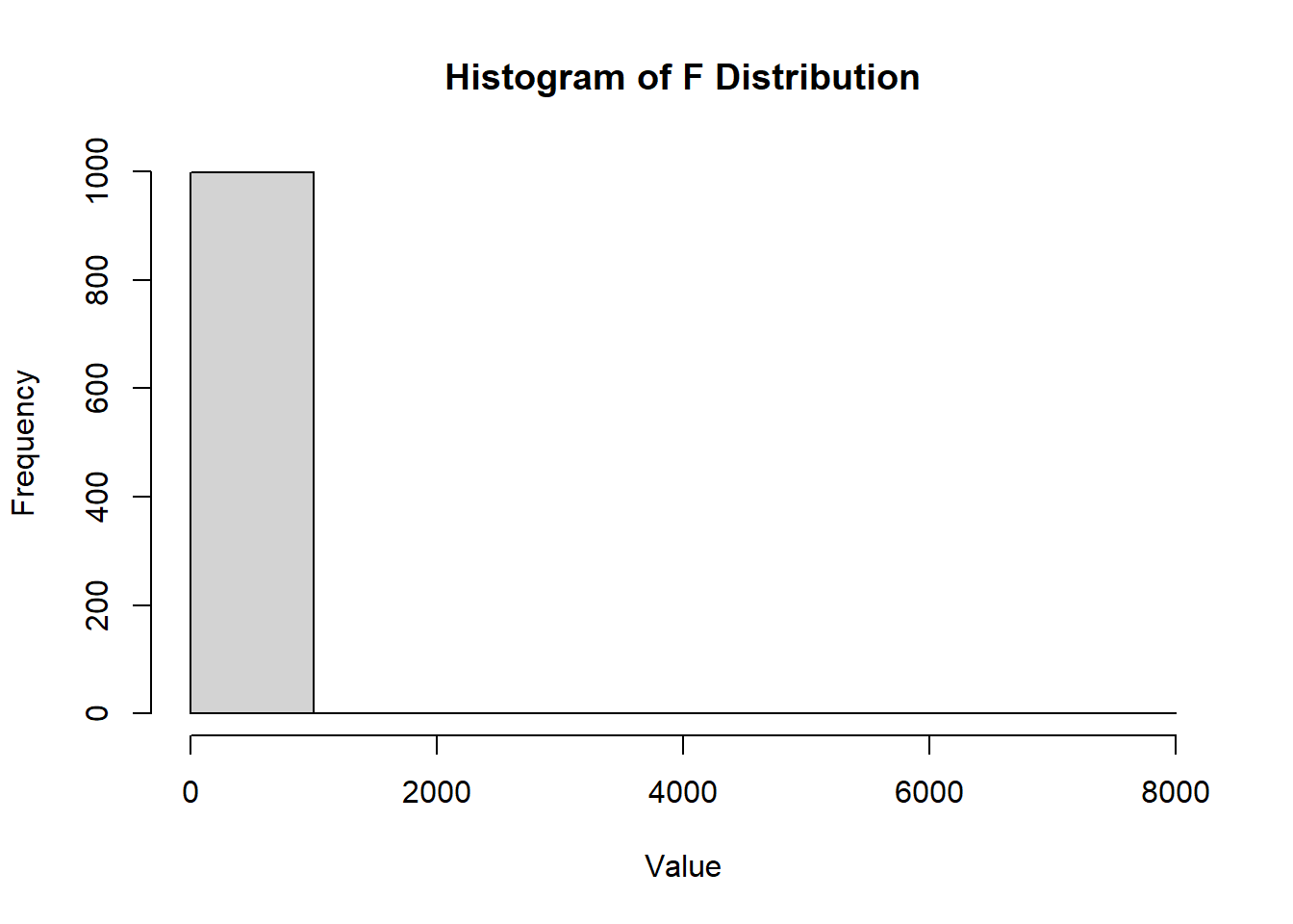
Figure 2.21: Histogram of MVN Distribution (1st Var)
MGF
\[ m_{\mathbf{X}}(\mathbf{t}) = \exp\left(\boldsymbol{\mu}^T \mathbf{t} + \frac{1}{2} \mathbf{t}^T \boldsymbol{\Sigma} \mathbf{t} \right) \]
Mean
\[ E[\mathbf{X}] = \boldsymbol{\mu} \]
Variance
\[ \text{Var}(\mathbf{X}) = \boldsymbol{\Sigma} \]
2.3 General Math
2.3.1 Number Sets
| Notation | Denotes | Examples |
|---|---|---|
| \(\emptyset\) | Empty set | No members |
| \(\mathbb{N}\) | Natural numbers | \(\{1, 2, \ldots\}\) |
| \(\mathbb{Z}\) | Integers | \(\{\ldots, -1, 0, 1, \ldots\}\) |
| \(\mathbb{Q}\) | Rational numbers | Including fractions |
| \(\mathbb{R}\) | Real numbers | Including all finite decimals, irrational numbers |
| \(\mathbb{C}\) | Complex numbers | Including numbers of the form \(a + bi\) where \(i^2 = -1\) |
2.3.2 Summation Notation and Series
2.3.2.1 Chebyshev’s Inequality
Let \(X\) be a random variable with mean \(\mu\) and standard deviation \(\sigma\). For any positive number \(k\), Chebyshev’s Inequality states:
\[ P(|X-\mu| \geq k\sigma) \leq \frac{1}{k^2} \]
This provides a probabilistic bound on the deviation of \(X\) from its mean and does not require \(X\) to follow a normal distribution.
2.3.2.2 Geometric Sum
For a geometric series of the form \(\sum_{k=0}^{n-1} ar^k\), the sum is given by:
\[ \sum_{k=0}^{n-1} ar^k = a\frac{1-r^n}{1-r} \quad \text{where } r \neq 1 \]
2.3.2.3 Infinite Geometric Series
When \(|r| < 1\), the geometric series converges to:
\[ \sum_{k=0}^\infty ar^k = \frac{a}{1-r} \]
2.3.2.4 Binomial Theorem
The binomial expansion for \((x + y)^n\) is:
\[ (x + y)^n = \sum_{k=0}^n \binom{n}{k} x^{n-k} y^k \quad \text{where } n \geq 0 \]
2.3.2.5 Binomial Series
For non-integer exponents \(\alpha\):
\[ \sum_{k=0}^\infty \binom{\alpha}{k} x^k = (1 + x)^\alpha \quad \text{where } |x| < 1 \]
2.3.2.6 Telescoping Sum
A telescoping sum simplifies as intermediate terms cancel, leaving:
\[ \sum_{a \leq k < b} \Delta F(k) = F(b) - F(a) \quad \text{where } a, b \in \mathbb{Z}, a \leq b \]
2.3.2.7 Vandermonde Convolution
The Vandermonde convolution identity is:
\[ \sum_{k=0}^n \binom{r}{k} \binom{s}{n-k} = \binom{r+s}{n} \quad \text{where } n \in \mathbb{Z} \]
2.3.2.8 Exponential Series
The exponential function \(e^x\) can be represented as:
\[ \sum_{k=0}^\infty \frac{x^k}{k!} = e^x \quad \text{where } x \in \mathbb{C} \]
2.3.2.9 Taylor Series
The Taylor series expansion for a function \(f(x)\) about \(x=a\) is:
\[ \sum_{k=0}^\infty \frac{f^{(k)}(a)}{k!} (x-a)^k = f(x) \]
For \(a = 0\), this becomes the Maclaurin series.
2.3.2.10 Maclaurin Series for \(e^z\)
A special case of the Taylor series, the Maclaurin expansion for \(e^z\) is:
\[ e^z = 1 + z + \frac{z^2}{2!} + \frac{z^3}{3!} + \cdots \]
2.3.2.11 Euler’s Summation Formula
Euler’s summation formula connects sums and integrals:
\[ \sum_{a \leq k < b} f(k) = \int_a^b f(x) dx + \sum_{k=1}^m \frac{B_k}{k!} \left[f^{(k-1)}(x)\right]_a^b + (-1)^{m+1} \int_a^b \frac{B_m(x-\lfloor x \rfloor)}{m!} f^{(m)}(x) dx \]
Here, \(B_k\) are Bernoulli numbers.
- For \(m=1\) (Trapezoidal Rule):
\[ \sum_{a \leq k < b} f(k) \approx \int_a^b f(x) dx - \frac{1}{2}(f(b) - f(a)) \]
2.3.3 Taylor Expansion
A differentiable function, \(G(x)\), can be written as an infinite sum of its derivatives. More specifically, if \(G(x)\) is infinitely differentiable and evaluated at \(a\), its Taylor expansion is:
\[ G(x) = G(a) + \frac{G'(a)}{1!} (x-a) + \frac{G''(a)}{2!}(x-a)^2 + \frac{G'''(a)}{3!}(x-a)^3 + \dots \]
This expansion is valid within the radius of convergence.
2.3.4 Law of Large Numbers
Let \(X_1, X_2, \ldots\) be an infinite sequence of independent and identically distributed (i.i.d.) random variables with finite mean \(\mu\) and variance \(\sigma^2\). The Law of Large Numbers (LLN) states that the sample average:
\[ \bar{X}_n = \frac{1}{n} \sum_{i=1}^n X_i \]
converges to the expected value \(\mu\) as \(n \rightarrow \infty\). This can be expressed as:
\[ \bar{X}_n \rightarrow \mu \quad \text{(as $n \rightarrow \infty$)}. \]
2.3.4.1 Variance of the Sample Mean
The variance of the sample mean decreases as the sample size increases:
\[ Var(\bar{X}_n) = Var\left(\frac{1}{n} \sum_{i=1}^n X_i\right) = \frac{\sigma^2}{n}. \]
\[ \begin{aligned} Var(\bar{X}_n) &= Var(\frac{1}{n}(X_1 + ... + X_n)) =Var\left(\frac{1}{n} \sum_{i=1}^n X_i\right) \\ &= \frac{1}{n^2}Var(X_1 + ... + X_n) \\ &=\frac{n\sigma^2}{n^2}=\frac{\sigma^2}{n} \end{aligned} \]
Note: The connection between the Law of Large Numbers and the Normal Distribution lies in the Central Limit Theorem. The CLT states that, regardless of the original distribution of a dataset, the distribution of the sample means will tend to follow a normal distribution as the sample size becomes larger.
The difference between [Weak Law] and [Strong Law] regards the mode of convergence.
2.3.4.2 Weak Law of Large Numbers
The Weak Law of Large Numbers states that the sample average converges in probability to the expected value:
\[ \bar{X}_n \xrightarrow{p} \mu \quad \text{as } n \rightarrow \infty. \]
Formally, for any \(\epsilon > 0\):
\[ \lim_{n \to \infty} P(|\bar{X}_n - \mu| > \epsilon) = 0. \]
Additionally, the sample mean of an i.i.d. random sample (\(\{ X_i \}_{i=1}^n\)) from any population with a finite mean and variance is a consistent estimator of the population mean \(\mu\):
\[ plim(\bar{X}_n) = plim\left(\frac{1}{n}\sum_{i=1}^{n} X_i\right) = \mu. \]
2.3.4.3 Strong Law of Large Numbers
The Strong Law of Large Numbers states that the sample average converges almost surely to the expected value:
\[ \bar{X}_n \xrightarrow{a.s.} \mu \quad \text{as } n \rightarrow \infty. \]
Equivalently, this can be expressed as:
\[ P\left(\lim_{n \to \infty} \bar{X}_n = \mu\right) = 1. \]
2.3.5 Convergence
2.3.5.1 Convergence in Probability
As \(n \rightarrow \infty\), an estimator (random variable) \(\theta_n\) is said to converge in probability to a constant \(c\) if:
\[ \lim_{n \to \infty} P(|\theta_n - c| \geq \epsilon) = 0 \quad \text{for any } \epsilon > 0. \]
This is denoted as:
\[ plim(\theta_n) = c \quad \text{or equivalently, } \theta_n \xrightarrow{p} c. \]
Properties of Convergence in Probability:
-
Slutsky’s Theorem: For a continuous function \(g(\cdot)\), if \(plim(\theta_n) = \theta\), then:
\[ plim(g(\theta_n)) = g(\theta) \]
-
If \(\gamma_n \xrightarrow{p} \gamma\), then:
- \(plim(\theta_n + \gamma_n) = \theta + \gamma\),
- \(plim(\theta_n \gamma_n) = \theta \gamma\),
- \(plim(\theta_n / \gamma_n) = \theta / \gamma\) (if \(\gamma \neq 0\)).
These properties extend to random vectors and matrices.
2.3.5.2 Convergence in Distribution
As \(n \rightarrow \infty\), the distribution of a random variable \(X_n\) may converge to another (“fixed”) distribution. Formally, \(X_n\) with CDF \(F_n(x)\) converges in distribution to \(X\) with CDF \(F(x)\) if:
\[ \lim_{n \to \infty} |F_n(x) - F(x)| = 0 \]
at all points of continuity of \(F(x)\). This is denoted as:
\[ X_n \xrightarrow{d} X \quad \text{or equivalently, } F(x) \text{ is the limiting distribution of } X_n. \]
Asymptotic Properties:
- \(E(X)\): Limiting mean (asymptotic mean).
- \(Var(X)\): Limiting variance (asymptotic variance).
Note: Limiting expectations and variances do not necessarily match the expectations and variances of \(X_n\):
\[ \begin{aligned} E(X) &\neq \lim_{n \to \infty} E(X_n), \\ Avar(X_n) &\neq \lim_{n \to \infty} Var(X_n). \end{aligned} \]
Properties of Convergence in Distribution:
-
Continuous Mapping Theorem: For a continuous function \(g(\cdot)\), if \(X_n \xrightarrow{d} X\), then:
\[ g(X_n) \xrightarrow{d} g(X). \]
-
If \(Y_n \xrightarrow{d} c\) (a constant), then:
- \(X_n + Y_n \xrightarrow{d} X + c\),
- \(Y_n X_n \xrightarrow{d} c X\),
- \(X_n / Y_n \xrightarrow{d} X / c\) (if \(c \neq 0\)).
These properties also extend to random vectors and matrices.
| Convergence in Probability | Convergence in Distribution |
|---|---|
| Slutsky’s Theorem: For a continuous \(g(\cdot)\), if \(plim(\theta_n) = \theta\), then \(plim(g(\theta_n)) = g(\theta)\) | Continuous Mapping Theorem: For a continuous \(g(\cdot)\), if \(X_n \xrightarrow{d} X\), then \(g(X_n) \xrightarrow{d} g(X)\) |
| If \(\gamma_n \xrightarrow{p} \gamma\), then: | If \(Y_n \xrightarrow{d} c\), then: |
| \(plim(\theta_n + \gamma_n) = \theta + \gamma\) | \(X_n + Y_n \xrightarrow{d} X + c\) |
| \(plim(\theta_n \gamma_n) = \theta \gamma\) | \(Y_n X_n \xrightarrow{d} c X\) |
| \(plim(\theta_n / \gamma_n) = \theta / \gamma\) (if \(\gamma \neq 0\)) | \(X_n / Y_n \xrightarrow{d} X / c\) (if \(c \neq 0\)) |
Relationship between Convergence Types:
Convergence in Probability is stronger than Convergence in Distribution. Therefore:
- Convergence in Distribution does not guarantee Convergence in Probability.
2.3.6 Sufficient Statistics and Likelihood
2.3.6.1 Likelihood
The likelihood describes the degree to which the observed data supports a particular value of a parameter \(\theta\).
- The exact value of the likelihood is not meaningful; only relative comparisons matter.
- Likelihood is informative when comparing parameter values, helping identify which values of \(\theta\) are more plausible given the data.
For a single observation \(Y = y\), the likelihood function is defined as:
\[ L(\theta_0; y) = P(Y = y \mid \theta = \theta_0) = f_Y(y; \theta_0), \]
where \(f_Y(y; \theta_0)\) is the probability density (or mass) function of \(Y\) for the parameter \(\theta_0\).
Key Insight: The likelihood tells us how plausible \(\theta\) is, given the data we observed. It is not a probability, but it is proportional to the probability of observing the data under a given parameter value.
Example: Suppose \(Y\) follows a binomial distribution with \(n=10\) trials and probability of success \(p\):
\[ P(Y = y \mid p) = \binom{10}{y} p^y (1-p)^{10-y}. \]
For \(y=7\) observed successes, the likelihood function becomes:
\[ L(p; y=7) = \binom{10}{7} p^7 (1-p)^3. \]
We can use this to compare how well different values of \(p\) explain the observed data.
2.3.6.2 Likelihood Ratio
The likelihood ratio compares the relative likelihood of two parameter values \(\theta_0\) and \(\theta_1\) given the observed data:
\[ \text{Likelihood Ratio} = \frac{L(\theta_0; y)}{L(\theta_1; y)}. \]
- A likelihood ratio greater than 1 implies that \(\theta_0\) is more likely than \(\theta_1\), given the observed data.
- Likelihood ratios are widely used in hypothesis testing and model comparison to evaluate the evidence against a null hypothesis.
Example: For the binomial example above, consider \(p_0 = 0.7\) and \(p_1 = 0.5\). The likelihood ratio is:
\[ \frac{L(p_0; y=7)}{L(p_1; y=7)} = \frac{\binom{10}{7} (0.7)^7 (0.3)^3}{\binom{10}{7} (0.5)^7 (0.5)^3}. \]
This simplifies to:
\[ \frac{(0.7)^7 (0.3)^3}{(0.5)^7 (0.5)^3}. \]
The likelihood ratio quantifies how much more likely \(p_0\) is compared to \(p_1\) given the observed data.
2.3.6.3 Likelihood Function
For a given sample, the likelihood for all possible values of \(\theta\) forms the likelihood function:
\[ L(\theta) = L(\theta; y) = f_Y(y; \theta). \]
For a sample of size \(n\), assuming independence among observations:
\[ L(\theta) = \prod_{i=1}^{n} f_Y(y_i; \theta). \]
Taking the natural logarithm of the likelihood gives the log-likelihood function:
\[ l(\theta) = \sum_{i=1}^{n} \log f_Y(y_i; \theta). \]
Why Log-Likelihood?
- The log-likelihood simplifies computation by turning products into sums.
- It is particularly useful for optimization, as many numerical methods (e.g., gradient-based algorithms) perform better with sums than products.
Example: For \(Y_1, Y_2, \dots, Y_n\) i.i.d. observations from a normal distribution \(N(\mu, \sigma^2)\), the likelihood is:
\[ L(\mu, \sigma^2) = \prod_{i=1}^n \frac{1}{\sqrt{2\pi\sigma^2}} \exp\left(-\frac{(y_i - \mu)^2}{2\sigma^2}\right). \]
The log-likelihood is:
\[ l(\mu, \sigma^2) = -\frac{n}{2} \log(2\pi\sigma^2) - \frac{1}{2\sigma^2} \sum_{i=1}^n (y_i - \mu)^2. \]
2.3.6.4 Sufficient Statistics
A sufficient statistic \(T(y)\) is a summary of the data that retains all information about a parameter \(\theta\). It allows us to focus on this condensed statistic without losing any inferential power regarding \(\theta\).
Formal Definition:
A statistic \(T(y)\) is sufficient for a parameter \(\theta\) if the conditional probability distribution of the data \(y\), given \(T(y)\) and \(\theta\), does not depend on \(\theta\). Mathematically:
\[ P(Y = y \mid T(y), \theta) = P(Y = y \mid T(y)). \]
Alternatively, by the Factorization Theorem, \(T(y)\) is sufficient if the likelihood can be written as:
\[ L(\theta; y) = c(y) L^*(\theta; T(y)), \]
where:
- \(c(y)\) is a function of the data independent of \(\theta\).
- \(L^*(\theta; T(y))\) is a function that depends on \(\theta\) and \(T(y)\).
In other words, the likelihood function can be rewritten in terms of \(T(y)\) alone, without loss of information about \(\theta\).
Why Sufficient Statistics Matter:
- They allow us to simplify the analysis by reducing the data without losing inferential power.
- Many inferential procedures (e.g., Maximum Likelihood Estimation, Bayesian methods) are simplified by working with sufficient statistics.
Example:
Consider a sample of i.i.d. observations \(Y_1, Y_2, \dots, Y_n\) from a normal distribution \(N(\mu, \sigma^2)\). Here:
- The sample mean \(\bar{Y} = \frac{1}{n} \sum_{i=1}^n Y_i\) is sufficient for \(\mu\).
- The sample variance \(S^2 = \frac{1}{n-1} \sum_{i=1}^n (Y_i - \bar{Y})^2\) is sufficient for \(\sigma^2\).
Verification: The joint density of \(y_1, y_2, \dots, y_n\) can be factored as:
\[ f(y_1, \dots, y_n; \mu, \sigma^2) = \underbrace{\frac{1}{(2\pi\sigma^2)^{n/2}} \exp\left(-\frac{1}{2\sigma^2} \sum_{i=1}^n (y_i - \bar{y})^2\right)}_{L^*(\mu, \sigma^2; \bar{y}, s^2)} \cdot \underbrace{\text{[independent of $\mu$, $\sigma^2$]}}_{c(y)}. \]
This shows \(\bar{Y}\) and \(S^2\) are sufficient.
Usage of Sufficient Statistics
-
Maximum Likelihood Estimation (MLE): In MLE, sufficient statistics simplify the optimization problem by reducing the data without losing information.
Example: In the normal distribution case, \(\mu\) can be estimated using the sufficient statistic \(\bar{Y}\): \[ \hat{\mu}_{MLE} = \bar{Y}. \]
Bayesian Inference: In Bayesian analysis, the posterior distribution depends on the sufficient statistic rather than the entire data set. For the normal case: \[ P(\mu \mid \bar{Y}) \propto P(\mu) L(\mu; \bar{Y}). \]
Data Compression: In practice, sufficient statistics reduce the complexity of data storage and analysis by condensing all relevant information into a smaller representation.
2.3.6.5 Nuisance Parameters
Parameters that are not of direct interest in the analysis but are necessary to model the data are called nuisance parameters.
Profile Likelihood: To handle nuisance parameters, replace them with their maximum likelihood estimates (MLEs) in the likelihood function, creating a profile likelihood for the parameter of interest.
Example of Profile Likelihood:
In a regression model with parameters \(\beta\) (coefficients) and \(\sigma^2\) (error variance), \(\sigma^2\) is often a nuisance parameter. The profile likelihood for \(\beta\) is obtained by substituting the MLE of \(\sigma^2\) into the likelihood:
\[ L_p(\beta) = L(\beta, \hat{\sigma}^2), \]
where \(\hat{\sigma}^2\) is the MLE of \(\sigma^2\) given \(\beta\).
This simplifies the problem to focus only on the parameter of interest, \(\beta\).
2.3.7 Parameter Transformations
Transformations of parameters are often used to improve interpretability or statistical properties of models.
2.3.7.1 Log-Odds Transformation
The log-odds transformation is commonly used in logistic regression and binary classification problems. It transforms probabilities (which are bounded between 0 and 1) to the real line:
\[ \text{Log odds} = g(\theta) = \ln\left(\frac{\theta}{1-\theta}\right), \]
where \(\theta\) represents a probability (e.g., the success probability in a Bernoulli trial).
2.3.7.2 General Parameter Transformations
For a parameter \(\theta\) and a transformation \(g(\cdot)\):
- If \(\theta \in (a, b)\), \(g(\theta)\) may map \(\theta\) to a different range (e.g., \(\mathbb{R}\)).
- Useful transformations include:
- Logarithmic: \(g(\theta) = \ln(\theta)\) for \(\theta > 0\).
- Exponential: \(g(\theta) = e^{\theta}\) for unconstrained \(\theta\).
- Square root: \(g(\theta) = \sqrt{\theta}\) for \(\theta \geq 0\).
Jacobian Adjustment for Transformations: If transforming a parameter in Bayesian inference, the Jacobian of the transformation must be included to ensure proper posterior scaling.
2.3.7.3 Applications of Parameter Transformations
-
Improving Interpretability:
- Probabilities can be transformed to odds or log-odds for logistic models.
- Rates can be transformed logarithmically for multiplicative effects.
-
Statistical Modeling:
- Variance-stabilizing transformations (e.g., log for Poisson data or arcsine for proportions).
- Regularization or simplification of complex relationships.
-
Optimization:
- Transforming constrained parameters (e.g., probabilities or positive scales) to unconstrained scales simplifies optimization algorithms.
2.4 Data Import/Export
R is a powerful and flexible tool for data analysis, but it was originally designed for in-memory statistical computing. This imposes several practical limitations, especially when handling large datasets.
2.4.1 Key Limitations of R
Single-Core Default Execution
By default, R utilizes only one CPU core, limiting performance for compute-intensive tasks unless parallelization is explicitly implemented.-
Memory-Based Data Handling
R loads data into RAM. This approach becomes problematic when working with datasets that exceed the available memory.- Medium-Sized Files: Fits within typical RAM (1–2 GB). Processing is straightforward.
- Large Files: Between 2–10 GB. May require memory-efficient coding or special packages.
- Very Large Files: Exceed 10 GB. Necessitates distributed or parallel computing solutions.
2.4.2 Solutions and Workarounds
- Upgrade Hardware
- Increase RAM: A simple but often effective solution for moderately large datasets.
- Leverage High-Performance Computing (HPC) in R
There are several HPC strategies and packages in R that facilitate working with large or computationally intensive tasks:
Explicit Parallelism
Use packages likeparallel,foreach,doParallel,future, andsnowto define how code runs across multiple cores or nodes.Implicit Parallelism
Certain functions in packages such asdata.table,dplyr, orcaretinternally optimize performance across cores when available.Large-Memory Computation
Use memory-efficient structures or external memory algorithms.MapReduce Paradigm
Useful in distributed computing environments, especially with big data infrastructure like Hadoop.
- Efficient Data Loading
- Limit Rows and Columns
Use arguments such asnrows =in functions likeread.csv()orfread()to load subsets of large datasets.
- Use Specialized Packages for Large Data
-
In-Memory Matrix Packages (Single Class Type Support)
These packages interface with C++ to handle large matrices more efficiently:-
bigmemory,biganalytics,bigtabulate,synchronicity,bigalgebra,bigvideo
-
-
Out-of-Memory Storage (Multiple Class Types)
For datasets with various data types:-
ffpackage: Stores data on disk and accesses it as needed, suitable for mixed-type columns.
-
- Handling Very Large Datasets (>10 GB)
When data size exceeds the capacity of a single machine, distributed computing becomes necessary:
- Hadoop Ecosystem Integration
-
RHadoop: A suite of R packages that integrate with the Hadoop framework. -
HadoopStreaming: Enables R scripts to be used as Hadoop mappers and reducers. -
Rhipe: Provides a more R-like interface to Hadoop, using Google’s Protocol Buffers for serialization.
-
2.4.3 Medium size
To import multiple files in a directory
str(import_list(dir()), which = 1)To export a single data file
export(data, "data.csv")
export(data,"data.dta")
export(data,"data.txt")
export(data,"data_cyl.rds")
export(data,"data.rdata")
export(data,"data.R")
export(data,"data.csv.zip")
export(data,"list.json")
To export multiple data files
export(list(mtcars = mtcars, iris = iris), "data_file_type")
# where data_file_type should substituted with the extension listed above
To convert between data file types
# convert Stata to SPSS
convert("data.dta", "data.sav")
2.4.4 Large size
2.4.4.1 Cloud Computing: Using AWS for Big Data
Amazon Web Service (AWS): Compute resources can be rented at approximately $1/hr. Use AWS to process large datasets without overwhelming your local machine.
2.4.4.2 Importing Large Files as Chunks
2.4.4.2.2 Using the data.table Package
library(data.table)
mydata <- fread("in.csv", header = TRUE)  # Fast and memory-efficient
2.4.4.2.4 Using the bigmemory Package
library(bigmemory)
my_data <- read.big.matrix('in.csv', header = TRUE)
2.4.4.2.5 Using the sqldf Package
library(sqldf)
my_data <- read.csv.sql('in.csv')

# Example: Filtering during import
iris2 <- read.csv.sql("iris.csv",
    sql = "SELECT * FROM file WHERE Species = 'setosa'")
2.4.4.2.6 Using the RMySQL Package
RQLite package
- Download SQLite, pick “A bundle of command-line tools for managing SQLite database files” for Window 10
- Unzip file, and open
sqlite3.exe. - Type in the prompt
-
sqlite> .cd 'C:\Users\data'specify path to your desired directory -
sqlite> .open database_name.dbto open a database - To import the CSV file into the database
-
sqlite> .mode csvspecify to SQLite that the next file is .csv file -
sqlite> .import file_name.csv datbase_nameto import the csv file to the database
-
-
sqlite> .exitAfter you’re done, exit the sqlite program
-
2.4.4.2.7 Using the arrow Package
library(arrow)
data <- read_csv_arrow("file.csv")
2.4.4.2.8 Using the vroom Package
library(vroom)

# Import a compressed CSV file
compressed <- vroom_example("mtcars.csv.zip")
data <- vroom(compressed)
2.4.4.2.9 Using the data.table Package
s = fread("sample.csv")2.4.4.2.10 Comparisons Regarding Storage Space
test = ff::read.csv.ffdf(file = "")
object.size(test) # Highest memory usage

test1 = data.table::fread(file = "")
object.size(test1) # Lowest memory usage

test2 = readr::read_csv(file = "")
object.size(test2) # Second lowest memory usage

test3 = vroom::vroom(file = "")
object.size(test3) # Similar to read_csv
When dealing with large datasets—especially those exceeding 10 GB—standard data-loading strategies in R can become impractical due to memory constraints. One common approach is to store these datasets in a compressed format such as .csv.gz, which saves disk space while preserving compatibility with many tools.
Compressed files (e.g., csv.gz) are especially useful for archiving and transferring large datasets. However, R typically loads the entire dataset into memory before writing or processing, which is inefficient or even infeasible for very large files.
In such cases, sequential processing becomes essential. Rather than reading the entire dataset at once, you can process it in chunks or rows, minimizing memory usage.
| Function | Supports Connections | Sequential Access | Performance | Notes |
|---|---|---|---|---|
read.csv() |
Yes | Yes | Slower | Base R; can work with gz-compressed files and allows looped reading |
readr::read_csv() |
Limited | No | Faster | High performance but re-reads lines even when using skip
|
While readr::read_csv() is faster and more efficient for smaller files, it has a limitation for large files when used with skip. The skip argument does not avoid reading the skipped rows—it simply discards them after reading. This leads to redundant I/O operations and significantly slows down performance for large files.
readr::read_csv(file, n_max = 100, skip = 0)        # Reads rows 1–100
readr::read_csv(file, n_max = 200, skip = 100)      # Re-reads rows 1–100, then reads 101–300
This approach is inefficient when processing data in chunks.
read.csv() can read directly from a file or a connection, and unlike readr::read_csv(), it maintains the connection state, allowing you to loop over chunks without re-reading prior rows.
Example: Sequential Reading with Connection
con <- gzfile("large_file.csv.gz", open = "rt")  # Text mode
headers <- read.csv(con, nrows = 1)              # Read column names
repeat {
  chunk <- tryCatch(read.csv(con, nrows = 1000), error = function(e) NULL)
  if (is.null(chunk) || nrow(chunk) == 0) break
  # Process 'chunk' here
}
close(con)
Occasionally, when reading compressed or encoded files, you might encounter the following error:
Error in (function (con, what, n = 1L, size = NA_integer_, signed = TRUE):
can only read from a binary connection
This can occur if the file is not correctly interpreted as text. A workaround is to explicitly set the connection mode to binary using "rb":
con <- gzfile("large_file.csv.gz", open = "rb") # Binary modeAlthough file() and gzfile() generally detect formats automatically, setting the mode explicitly can resolve issues when the behavior is inconsistent.
2.5 Data Manipulation
# Load required packages
library(tidyverse)
library(lubridate)

# -----------------------------
# Data Structures in R
# -----------------------------

# Create vectors
x <- c(1, 4, 23, 4, 45)
n <- c(1, 3, 5)
g <- c("M", "M", "F")

# Create a data frame
df <- data.frame(n, g)
df  # View the data frame
#>   n g
#> 1 1 M
#> 2 3 M
#> 3 5 F
str(df)  # Check its structure
#> 'data.frame':    3 obs. of  2 variables:
#>  $ n: num  1 3 5
#>  $ g: chr  "M" "M" "F"

# Using tibble for cleaner outputs
df <- tibble(n, g)
df  # View the tibble
#> # A tibble: 3 × 2
#>       n g
#>   <dbl> <chr>
#> 1     1 M
#> 2     3 M
#> 3     5 F
str(df)
#> tibble [3 × 2] (S3: tbl_df/tbl/data.frame)
#>  $ n: num [1:3] 1 3 5
#>  $ g: chr [1:3] "M" "M" "F"

# Create a list
lst <- list(x, n, g, df)
lst  # Display the list
#> [[1]]
#> [1]  1  4 23  4 45
#>
#> [[2]]
#> [1] 1 3 5
#>
#> [[3]]
#> [1] "M" "M" "F"
#>
#> [[4]]
#> # A tibble: 3 × 2
#>       n g
#>   <dbl> <chr>
#> 1     1 M
#> 2     3 M
#> 3     5 F

# Name list elements
lst2 <- list(num = x, size = n, sex = g, data = df)
lst2  # Named list elements are easier to reference
#> $num
#> [1]  1  4 23  4 45
#>
#> $size
#> [1] 1 3 5
#>
#> $sex
#> [1] "M" "M" "F"
#>
#> $data
#> # A tibble: 3 × 2
#>       n g
#>   <dbl> <chr>
#> 1     1 M
#> 2     3 M
#> 3     5 F

# Another list example with numeric vectors
lst3 <- list(
  x = c(1, 3, 5, 7),
  y = c(2, 2, 2, 4, 5, 5, 5, 6),
  z = c(22, 3, 3, 3, 5, 10)
)
lst3
#> $x
#> [1] 1 3 5 7
#>
#> $y
#> [1] 2 2 2 4 5 5 5 6
#>
#> $z
#> [1] 22  3  3  3  5 10

# Find means of list elements
# One at a time
mean(lst3$x)
#> [1] 4
mean(lst3$y)
#> [1] 3.875
mean(lst3$z)
#> [1] 7.666667

# Using lapply to calculate means
lapply(lst3, mean)
#> $x
#> [1] 4
#>
#> $y
#> [1] 3.875
#>
#> $z
#> [1] 7.666667

# Simplified output with sapply
sapply(lst3, mean)
#>        x        y        z
#> 4.000000 3.875000 7.666667

# Tidyverse alternative: map() function
map(lst3, mean)
#> $x
#> [1] 4
#>
#> $y
#> [1] 3.875
#>
#> $z
#> [1] 7.666667

# Tidyverse with numeric output: map_dbl()
map_dbl(lst3, mean)
#>        x        y        z
#> 4.000000 3.875000 7.666667

# -----------------------------
# Binding Data Frames
# -----------------------------

# Create tibbles for demonstration
dat01 <- tibble(x = 1:5, y = 5:1)
dat02 <- tibble(x = 10:16, y = x / 2)
dat03 <- tibble(z = runif(5))  # 5 random numbers from (0, 1)

# Row binding
bind_rows(dat01, dat02, dat01)
#> # A tibble: 17 × 2
#>        x     y
#>    <int> <dbl>
#>  1     1   5
#>  2     2   4
#>  3     3   3
#>  4     4   2
#>  5     5   1
#>  6    10   5
#>  7    11   5.5
#>  8    12   6
#>  9    13   6.5
#> 10    14   7
#> 11    15   7.5
#> 12    16   8
#> 13     1   5
#> 14     2   4
#> 15     3   3
#> 16     4   2
#> 17     5   1

# Add a new identifier column with .id
bind_rows(dat01, dat02, .id = "id")
#> # A tibble: 12 × 3
#>    id        x     y
#>    <chr> <int> <dbl>
#>  1 1         1   5
#>  2 1         2   4
#>  3 1         3   3
#>  4 1         4   2
#>  5 1         5   1
#>  6 2        10   5
#>  7 2        11   5.5
#>  8 2        12   6
#>  9 2        13   6.5
#> 10 2        14   7
#> 11 2        15   7.5
#> 12 2        16   8

# Use named inputs for better identification
bind_rows("dat01" = dat01, "dat02" = dat02, .id = "id")
#> # A tibble: 12 × 3
#>    id        x     y
#>    <chr> <int> <dbl>
#>  1 dat01     1   5
#>  2 dat01     2   4
#>  3 dat01     3   3
#>  4 dat01     4   2
#>  5 dat01     5   1
#>  6 dat02    10   5
#>  7 dat02    11   5.5
#>  8 dat02    12   6
#>  9 dat02    13   6.5
#> 10 dat02    14   7
#> 11 dat02    15   7.5
#> 12 dat02    16   8

# Bind a list of data frames
list01 <- list("dat01" = dat01, "dat02" = dat02)
bind_rows(list01, .id = "source")
#> # A tibble: 12 × 3
#>    source     x     y
#>    <chr>  <int> <dbl>
#>  1 dat01      1   5
#>  2 dat01      2   4
#>  3 dat01      3   3
#>  4 dat01      4   2
#>  5 dat01      5   1
#>  6 dat02     10   5
#>  7 dat02     11   5.5
#>  8 dat02     12   6
#>  9 dat02     13   6.5
#> 10 dat02     14   7
#> 11 dat02     15   7.5
#> 12 dat02     16   8

# Column binding
bind_cols(dat01, dat03)
#> # A tibble: 5 × 3
#>       x     y     z
#>   <int> <int> <dbl>
#> 1     1     5 0.960
#> 2     2     4 0.357
#> 3     3     3 0.883
#> 4     4     2 0.123
#> 5     5     1 0.628

# -----------------------------
# String Manipulation
# -----------------------------

names <- c("Ford, MS", "Jones, PhD", "Martin, Phd", "Huck, MA, MLS")

# Remove everything after the first comma
str_remove(names, pattern = ", [[:print:]]+")
#> [1] "Ford"   "Jones"  "Martin" "Huck"

# Explanation: [[:print:]]+ matches one or more printable characters

# -----------------------------
# Reshaping Data
# -----------------------------

# Wide format data
wide <- data.frame(
  name = c("Clay", "Garrett", "Addison"),
  test1 = c(78, 93, 90),
  test2 = c(87, 91, 97),
  test3 = c(88, 99, 91)
)

# Long format data
long <- data.frame(
  name = rep(c("Clay", "Garrett", "Addison"), each = 3),
  test = rep(1:3, 3),
  score = c(78, 87, 88, 93, 91, 99, 90, 97, 91)
)

# Summary statistics
aggregate(score ~ name, data = long, mean)  # Mean score per student
#>      name    score
#> 1 Addison 92.66667
#> 2    Clay 84.33333
#> 3 Garrett 94.33333
aggregate(score ~ test, data = long, mean)  # Mean score per test
#>   test    score
#> 1    1 87.00000
#> 2    2 91.66667
#> 3    3 92.66667
# Line plot of scores over tests
ggplot(long,
       aes(
           x = factor(test),
           y = score,
           color = name,
           group = name
       )) +
    geom_point() +
    geom_line() +
    xlab("Test") +
    ggtitle("Test Scores by Student")
Figure 2.22: Test Scores by Student
# Reshape wide to long
pivot_longer(wide, test1:test3, names_to = "test", values_to = "score")
#> # A tibble: 9 × 3
#>   name    test  score
#>   <chr>   <chr> <dbl>
#> 1 Clay    test1    78
#> 2 Clay    test2    87
#> 3 Clay    test3    88
#> 4 Garrett test1    93
#> 5 Garrett test2    91
#> 6 Garrett test3    99
#> 7 Addison test1    90
#> 8 Addison test2    97
#> 9 Addison test3    91

# Use names_prefix to clean column names
pivot_longer(
    wide,
    -name,
    names_to = "test",
    values_to = "score",
    names_prefix = "test"
)
#> # A tibble: 9 × 3
#>   name    test  score
#>   <chr>   <chr> <dbl>
#> 1 Clay    1        78
#> 2 Clay    2        87
#> 3 Clay    3        88
#> 4 Garrett 1        93
#> 5 Garrett 2        91
#> 6 Garrett 3        99
#> 7 Addison 1        90
#> 8 Addison 2        97
#> 9 Addison 3        91

# Reshape long to wide with explicit id_cols argument
pivot_wider(
  long,
  id_cols = name,
  names_from = test,
  values_from = score
)
#> # A tibble: 3 × 4
#>   name      `1`   `2`   `3`
#>   <chr>   <dbl> <dbl> <dbl>
#> 1 Clay       78    87    88
#> 2 Garrett    93    91    99
#> 3 Addison    90    97    91

# Add a prefix to the resulting columns
pivot_wider(
  long,
  id_cols = name,
  names_from = test,
  values_from = score,
  names_prefix = "test"
)
#> # A tibble: 3 × 4
#>   name    test1 test2 test3
#>   <chr>   <dbl> <dbl> <dbl>
#> 1 Clay       78    87    88
#> 2 Garrett    93    91    99
#> 3 Addison    90    97    91
The verbs of data manipulation
-
select: selecting (or not selecting) columns based on their names (eg: select columns Q1 through Q25) -
slice: selecting (or not selecting) rows based on their position (eg: select rows 1:10) -
mutate: add or derive new columns (or variables) based on existing columns (eg: create a new column that expresses measurement in cm based on existing measure in inches) -
rename: rename variables or change column names (eg: change “GraduationRate100” to “grad100”) -
filter: selecting rows based on a condition (eg: all rows where gender = Male) -
arrange: ordering rows based on variable(s) numeric or alphabetical order (eg: sort in descending order of Income) -
sample: take random samples of data (eg: sample 80% of data to create a “training” set) -
summarize: condense or aggregate multiple values into single summary values (eg: calculate median income by age group) -
group_by: convert a tbl into a grouped tbl so that operations are performed “by group”; allows us to summarize data or apply verbs to data by groups (eg, by gender or treatment) - the pipe:
%>%Use Ctrl + Shift + M (Win) or Cmd + Shift + M (Mac) to enter in RStudio
The pipe takes the output of a function and “pipes” into the first argument of the next function.
new pipe is
|>It should be identical to the old one, except for certain special cases.
-
:=(Walrus operator): similar to=, but for cases where you want to use thegluepackage (i.e., dynamic changes in the variable name in the left-hand side)
Writing function in R
Tunneling
{{ (called curly-curly) allows you to tunnel data-variables through arg-variables (i.e., function arguments)
library(tidyverse)
# -----------------------------
# Writing Functions with {{ }}
# -----------------------------

# Define a custom function using {{ }}
get_mean <- function(data, group_var, var_to_mean) {
  data %>%
    group_by({{group_var}}) %>%
    summarize(mean = mean({{var_to_mean}}, na.rm = TRUE))
}

# Apply the function
data("mtcars")
mtcars %>%
  get_mean(group_var = cyl, var_to_mean = mpg)
#> # A tibble: 3 × 2
#>     cyl  mean
#>   <dbl> <dbl>
#> 1     4  26.7
#> 2     6  19.7
#> 3     8  15.1

# Dynamically name the resulting variable
get_mean <- function(data, group_var, var_to_mean, prefix = "mean_of") {
  data %>%
    group_by({{group_var}}) %>%
    summarize("{prefix}_{{var_to_mean}}" := mean({{var_to_mean}}, na.rm = TRUE))
}

# Apply the modified function
mtcars %>%
  get_mean(group_var = cyl, var_to_mean = mpg)
#> # A tibble: 3 × 2
#>     cyl mean_of_mpg
#>   <dbl>       <dbl>
#> 1     4        26.7
#> 2     6        19.7
#> 3     8        15.1