38 Directed Acyclic Graphs

Directed Acyclic Graphs (DAGs) provide a formal and visual framework for representing assumptions about causal structures. In modern data analysis, they are essential tools for understanding, identifying, and validating causal effects.

A DAG is a graph composed of nodes (representing variables) and directed edges (arrows) showing the direction of causality. “Acyclic” means that the graph contains no feedback loops; you cannot return to the same node by following the direction of the arrows.

Understanding DAGs helps analysts reason about:

• Which variables to control for in a regression model
• How to avoid collider bias and confounding
• What types of data are needed to estimate causal effects
• Where causal identification fails due to unobserved variables

These R packages facilitate DAG creation, visualization, and causal analysis:

• dagitty: Powerful syntax for defining DAGs, checking d-separation, and performing adjustment set analysis.
• ggdag: A ggplot2-based visualization tool for DAGs, compatible with dagitty, providing publication-ready DAGs.
• dagR: Focuses on applied epidemiological use of DAGs, particularly for teaching.
• r-causal: Developed by the Center for Causal Discovery. Offers methods for causal discovery from data (also in Python).

Web Tools

• Publication-ready DAG editor: shinyDAG – An R-based Shiny app for creating beautiful DAGs interactively.
• Standalone DAG tool: DAG program by Sven Knüppel – Excellent for beginners needing an intuitive graphical interface.

38.1 Basic Notation and Graph Structures

Directed Acyclic Graphs are composed of basic building blocks that define relationships between variables.

1. Mediators (Chains)

$$X \to Z \to Y$$

• Variable $Z$ mediates the effect of $X$ on $Y$.
• Controlling for $Z$ blocks the indirect effect of $X$ on $Y$.
• Use case in marketing: Email promotion ($X$) → customer interest ($Z$) → purchase ($Y$). Controlling for interest removes the indirect path, isolating the direct impact.

2. Common Causes (Forks)

$$X \leftarrow Z \to Y$$

• $Z$ is a confounder, creating a spurious association between $X$ and $Y$.
• To estimate the causal effect of $X$ on $Y$, $Z$ must be controlled.
• Use case in finance: An economic indicator ($Z$) affects both stock investment decisions ($X$) and market returns ($Y$).

Key concept: If $Z$ is not controlled, $X$ and $Y$ may appear correlated due to a shared cause rather than a causal link.

3. Common Effects (Colliders)

$$X \to Z \leftarrow Y$$

• $Z$ is a collider, and controlling for it induces a spurious association between $X$ and $Y$.
• Do not control for $Z$ or its descendants.
• Use case in HR analytics: Two independent hiring factors ($X$ = education, $Y$ = experience) both influence a decision variable $Z$ (hiring outcome). Conditioning on being hired can create an artificial correlation between education and experience.

Other Concepts

• Descendants: Any variable downstream from a node; controlling for a descendant can have similar effects to controlling for the ancestor.
• d-Separation: A graphical criterion to determine conditional independence. If all paths between $X$ and $Y$ are blocked by controlling for a set of variables $Z$, then $X$ is d-separated from $Y$ given $Z$.

38.2 Rule of Thumb for Causal Inference

To validly estimate the causal effect $X \to Y$:

• Close all backdoor paths between $X$ and $Y$ (paths that start with an arrow into $X$). This removes confounding.
• Do not block any part of the direct or indirect causal path from $X$ to $Y$ (especially via mediators).

This is known as the backdoor criterion—a formal condition from Pearl’s Causal Inference framework.

38.3 Example DAG

library(dagitty)
library(ggdag)

dag <- dagitty("dag {
  X -> Z -> Y
  Z <- U -> Y
}")

coordinates(dag) <- list(
  x = c(X = 1, Z = 2, Y = 3, U = 1.5),
  y = c(X = 1, Z = 1, Y = 1, U = 2)
)

ggdag(dag) +
  theme_dag()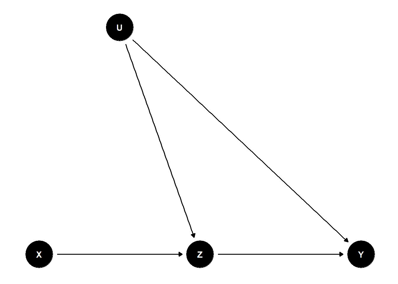

This DAG has:

• A mediator path: $X \to Z \to Y$
• A backdoor path through an unobserved confounder: $X \leftarrow U \to Y$

Use adjustmentSets(dag, exposure = "X", outcome = "Y") to identify a valid adjustment set.

38.4 Causal Discovery

Causal discovery involves algorithmically identifying causal relationships from data under a set of assumptions (like faithfulness and causal sufficiency). Key algorithms include:

• PC algorithm: Constraint-based, uses conditional independence testing
• GES (Greedy Equivalence Search): Score-based method
• FCI (Fast Causal Inference): Extends PC to handle latent confounders

See (Eberhardt, Kaynar, and Siddiq 2024) for a comprehensive discussion on the assumptions and limitations of discovery algorithms in practice.

38.5