17 Marginal Effects
Marginal effects play a fundamental role in interpreting regression models, particularly when analyzing the impact of explanatory variables on an outcome variable. These effects provide a precise measure of how a small change in an independent variable influences the dependent variable.
The concept of a marginal effect is closely linked to derivatives in calculus. In simple linear models, marginal effects correspond directly to the estimated regression coefficients. However, in nonlinear models, computing marginal effects requires careful consideration, often involving either analytical differentiation or numerical approximation.
17.1 Definition of Marginal Effects
Mathematically, the marginal effect of an independent variable \(X\) on the expected value of a dependent variable \(Y\) is given by:
\[ \frac{\partial E[Y|X]}{\partial X} \]
which represents the instantaneous rate of change of \(E[Y|X]\) with respect to \(X\).
For a linear regression model:
\[ Y = \beta_0 + \beta_1 X_1 + \beta_2 X_2 + \dots + \beta_k X_k + \varepsilon \]
the marginal effect of \(X_j\) is simply \(\beta_j\). However, in more complex cases, such as nonlinear models, interaction effects, or transformations, marginal effects are not directly given by the regression coefficients and must be computed explicitly.
17.1.1 Analytical Derivation of Marginal Effects
In models where \(E[Y|X]\) is a differentiable function of \(X\), marginal effects are computed using calculus. The derivative of a function \(f(x)\) is given by:
\[ f'(x) \equiv \lim_{h \to 0} \frac{f(x+h) - f(x)}{h} \]
Example: Quadratic Function
Consider the function:
\[ f(x) = x^2. \]
The marginal effect is derived as follows:
\[ \begin{aligned} f'(x) &= \lim_{h \to 0} \frac{(x+h)^2 - x^2}{h} \\ &= \frac{x^2 + 2xh + h^2 - x^2}{h} \\ &= \frac{2xh + h^2}{h} \\ &= 2x + h. \end{aligned} \]
As \(h \to 0\), the marginal effect simplifies to:
\[ f'(x) = 2x. \]
Thus, for small changes in \(x\), the effect on \(f(x)\) depends on \(x\) itself.
17.1.2 Numerical Approximation of Marginal Effects
In practice, analytical differentiation may be infeasible, particularly when dealing with complex functions, large datasets, or models without closed-form derivatives. In such cases, numerical differentiation provides an alternative.
17.1.2.1 One-Sided Numerical Approximation
A simple way to approximate the derivative is the forward difference formula:
\[ \begin{aligned} f'(x) &= \lim_{h \to 0} \frac{(x+h)^2 - x^2}{h} \\ & \approx \frac{f(x+h) -f(x)}{h} \end{aligned} \]
where \(h\) is a small step size.
17.1.2.2 Two-Sided Numerical Approximation
A more accurate method is the central difference formula:
\[ f'_2(x) \approx \frac{f(x+h) - f(x-h)}{2h}. \]
This approach reduces numerical error and is generally preferred in computational implementations.
17.1.2.3 Choosing an Appropriate \(h\)
The choice of \(h\) is critical (Gould, Pitblado, and Poi 2010, chap. 1):
- Too small: Can lead to numerical instability due to floating-point precision limitations.
- Too large: Reduces the accuracy of the approximation.
A common heuristic is to set \(h = 10^{-5}\) or a small fraction of the standard deviation of \(X\).
| Method | Advantages | Disadvantages |
|---|---|---|
| Analytical | Provides exact expressions | Requires differentiability, not always feasible |
| Numerical | Works for any function, easy to implement | Requires careful choice of step size \(h\) |
Numerical derivatives are often preferred in empirical applications, especially when working with complex models or machine learning algorithms.
| Analytical Derivation | Numerical Approximation | |
|---|---|---|
| Marginal Effects | Uses calculus (rules of differentiation) | Uses finite differences to approximate derivatives |
| Standard Errors | Derived using variance rules | Estimated via the delta method using the variance-covariance matrix |
17.2 Marginal Effects in Different Contexts
- Linear Regression Models
For a simple linear regression:
\[ E[Y|X] = \beta_0 + \beta_1 X, \]
the marginal effect is constant and equal to \(\beta_1\). This makes interpretation straightforward.
- Logit and Probit Models
In logistic regression, the expected value of \(Y\) is modeled as:
\[ E[Y|X] = P(Y=1|X) = \frac{1}{1 + e^{-\beta_0 - \beta_1 X}}. \]
The marginal effect is given by:
\[ \frac{\partial E[Y|X]}{\partial X} = \beta_1 P(Y=1|X) (1 - P(Y=1|X)). \]
Unlike linear models, the effect varies with \(X\), requiring evaluation at specific values (e.g., means or percentiles).
- Interaction Effects and Nonlinear Terms
When models include interactions (e.g., \(X_1 X_2\)) or transformations (e.g., \(\log(X)\)), marginal effects become more complex. For example, in:
\[ E[Y|X] = \beta_0 + \beta_1 X + \beta_2 X^2, \]
the marginal effect of \(X\) is:
\[ \frac{\partial E[Y|X]}{\partial X} = \beta_1 + 2\beta_2 X. \]
This means the marginal effect depends on the value of \(X\).
17.3 Marginal Effects Interpretation
The interpretation of marginal effects differs depending on whether \(X\) is continuous or discrete:
| Variable Type | Definition of Marginal Effect |
|---|---|
| Continuous | The derivative \(\frac{\partial E[Y|X]}{\partial X}\) represents an infinitesimal change in \(X\). |
| Discrete | The change in \(E[Y|X]\) when \(X\) increases by one unit (also called an incremental effect). |
For example, in a binary variable case (e.g., a dummy variable for gender), the marginal effect is:
\[ E[Y|X=1] - E[Y|X=0]. \]
which quantifies the expected change in \(Y\) when switching from \(X = 0\) to \(X = 1\).
17.4 Delta Method
The Delta Method is a statistical technique for approximating the mean and variance of a function of random variables. It is particularly useful in regression analysis when estimating the standard errors of nonlinear functions of estimated coefficients, such as:
- Marginal effects in nonlinear models (e.g., logistic regression)
- Elasticities and risk measures (e.g., in finance)
- Transformation of regression coefficients (e.g., log transformations)
This method is based on a first-order Taylor Series approximation, which allows us to estimate the variance of a transformed parameter without requiring explicit distributional assumptions.
Let \(G(\beta)\) be a function of the estimated parameters \(\beta\), where \(\beta\) follows an asymptotically normal distribution:
\[ \beta \sim N(\hat{\beta}, \text{Var}(\hat{\beta})). \]
Using a first-order Taylor expansion, we approximate \(G(\beta)\) around its expectation:
\[ G(\beta) \approx G(\hat{\beta}) + \nabla G(\beta) (\beta - \hat{\beta}), \]
where \(\nabla G(\beta)\) is the gradient (also known as the Jacobian) of \(G(\beta)\), i.e., the vector of partial derivatives:
\[ \nabla G(\beta) = \left( \frac{\partial G}{\partial \beta_1}, \frac{\partial G}{\partial \beta_2}, \dots, \frac{\partial G}{\partial \beta_k} \right). \]
The variance of \(G(\beta)\) is then approximated as:
\[ \text{Var}(G(\beta)) \approx \nabla G(\beta) \text{Cov}(\beta) \nabla G(\beta)'. \]
where:
\(\nabla G(\beta)\) is the gradient vector of \(G(\beta)\).
\(\text{Cov}(\beta)\) is the variance-covariance matrix of \(\hat{\beta}\).
The expression \(\nabla G(\beta)'\) denotes the transpose of the gradient.
Key Properties of the Delta Method
- Semi-parametric approach: It does not require full knowledge of the distribution of \(G(\beta)\).
- Widely applicable: Useful for computing standard errors in regression models.
-
Alternative approaches:
- Analytical derivation: Directly deriving a probability function for the margin.
- Simulation/Bootstrapping: Using Monte Carlo methods to approximate standard errors.
17.5 Comparison: Delta Method vs. Alternative Approaches
| Method | Description | Pros | Cons |
|---|---|---|---|
| Delta Method | Uses Taylor expansion to approximate variance | Computationally efficient | Accuracy depends on linearity assumption |
| Analytical Derivation | Directly derives probability function | Exact solution (if feasible) | Can be mathematically complex |
| Simulation/Bootstrapping | Uses repeated sampling from estimated distribution | No assumptions on functional form | Computationally expensive |
When to Use the Delta Method:
When you need a quick approximation for standard errors.
When the function \(G(\beta)\) is smooth and differentiable.
When working with large sample sizes, where asymptotic normality holds.
For deeper exploration, refer to these excellent resources:
Advanced: modmarg package documentation – covers implementation of the Delta Method in R.
Intermediate: UCLA Statistical Consulting – a practical FAQ on the Delta Method.
17.5.1 Example: Applying the Delta Method in a logistic regression
To illustrate, let’s apply the Delta Method to compute the standard error of a nonlinear transformation of regression coefficients.
In logistic regression, the estimated coefficient \(\hat{\beta}\) represents the log-odds change for a one-unit increase in \(X\). However, we often want the odds ratio, which is:
\[ G(\beta) = e^{\beta}. \]
By the Delta Method, the variance of \(e^{\beta}\) is:
\[ \text{Var}(e^{\beta}) \approx e^{2\beta} \cdot \text{Var}(\beta). \]
# Load necessary packages
library(ggplot2)
library(margins)
library(sandwich)
library(lmtest)

# Simulate data
set.seed(123)
n <- 100
X <- rnorm(n)  # Simulate independent variable
# Generate binary outcome using logistic model
Y <-
    rbinom(n, 1, plogis(0.5 + 0.8 * X))

# Logistic regression
logit_model <- glm(Y ~ X, family = binomial(link = "logit"))

# Extract coefficient and variance
beta_hat <- coef(logit_model)["X"]   # Estimated coefficient
var_beta_hat <- vcov(logit_model)["X", "X"]  # Variance of beta_hat

# Apply Delta Method
odds_ratio <- exp(beta_hat)  # Transform beta to odds ratio
se_odds_ratio <-
    sqrt(odds_ratio ^ 2 * var_beta_hat)  # Delta Method SE

# Compute 95% Confidence Interval
lower_CI <- exp(beta_hat - 1.96 * sqrt(var_beta_hat))
upper_CI <- exp(beta_hat + 1.96 * sqrt(var_beta_hat))

# Display results
results <- data.frame(
    Term = "X",
    Odds_Ratio = odds_ratio,
    SE = se_odds_ratio,
    Lower_CI = lower_CI,
    Upper_CI = upper_CI
)

print(results)
#>   Term Odds_Ratio        SE Lower_CI Upper_CI
#> X    X   2.655431 0.7677799 1.506669 4.680069

# ---- VISUALIZATION 1: Distribution of Simulated Odds Ratios ----
set.seed(123)
# Simulate beta estimates
simulated_betas <-
    rnorm(1000, mean = beta_hat, sd = sqrt(var_beta_hat))
simulated_odds_ratios <-
    exp(simulated_betas)  # Apply transformation
ggplot(data.frame(Odds_Ratio = simulated_odds_ratios),
       aes(x = Odds_Ratio)) +
    geom_histogram(
        color = "black",
        fill = "skyblue",
        bins = 50,
        alpha = 0.7
    ) +
    geom_vline(
        xintercept = odds_ratio,
        color = "red",
        linetype = "dashed",
        linewidth = 1.2
    ) +
    geom_vline(
        xintercept = lower_CI,
        color = "blue",
        linetype = "dotted",
        linewidth = 1.2
    ) +
    geom_vline(
        xintercept = upper_CI,
        color = "blue",
        linetype = "dotted",
        linewidth = 1.2
    ) +
    labs(title = "Distribution of Simulated Odds Ratios",
         x = "Odds Ratio",
         y = "Frequency") +
    theme_minimal()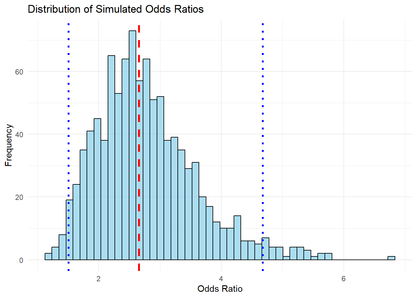
Figure 17.1: Distribution of Simulated Odds Ratios
-
Odds Ratio Computation
The odds ratio is the exponentiated coefficient \(e^{\hat{\beta}}\), which represents the multiplicative change in the odds of \(Y = 1\) for a one-unit increase in \(X\).
If \(\hat{\beta} = 0.8\), then \(e^{0.8} \approx 2.23\), meaning a one-unit increase in \(X\) increases the odds of \(Y = 1\) by 123%.
-
Standard Error via Delta Method
Since \(\beta\) follows a normal distribution, its transformation \(e^\beta\) is not normally distributed but rather follows a log-normal shape.
The Delta Method approximates the standard error of \(e^\beta\) using: \[ SE(e^\beta) = \sqrt{e^{2\beta} \cdot \text{Var}(\beta)} \]
-
Confidence Intervals
- The confidence interval is obtained by: \[ [e^{\beta - 1.96 \cdot SE}, e^{\beta + 1.96 \cdot SE}] \]
- This helps interpret the uncertainty around the odds ratio estimate.
-
Visualization
-
The histogram of simulated odds ratios shows how the transformation affects variance:
The red dashed line represents the estimated odds ratio.
The blue dotted lines show the confidence interval bounds.
The right-skewed distribution reflects the non-linear transformation, meaning higher uncertainty for larger values.
-
17.6 Types of Marginal Effect
17.6.1 Average Marginal Effect
The Average Marginal Effect (AME) measures the expected change in the predicted probability when an independent variable increases by a small amount while holding all other variables constant. Unlike marginal effects at the mean (MEM), AMEs average the marginal effects across all observations, providing a more representative measure.
Applications of AMEs
- Marketing: How much does increasing ad spend change the probability of a customer purchase?
- Finance: How does an interest rate change impact the probability of loan approval?
- Econometrics: What is the effect of education on the probability of employment?
Since nonlinear models like logit and probit do not have constant marginal effects, AMEs require numerical differentiation. There are two common approaches:
- One-Sided Numerical Derivative: Uses a small forward step \(h\) to estimate the derivative.
- Two-Sided Numerical Derivative: Takes both a forward step and a backward step to improve accuracy.
17.6.1.1 One-Sided Numerical Derivative
To estimate \(\frac{\partial p(\mathbf{X},\beta)}{\partial X}\) numerically:
Algorithm
- Estimate the model using logistic (or probit) regression.
- For each observation \(i\):
- Compute predicted probability using the observed data: \[ \hat{Y}_{i0} = p(\mathbf{X}_i, \hat{\beta}). \]
- Increase \(X\) by a small step \(h\), where:
- If \(X\) is continuous, choose:
\[ h = (|\bar{X}| + 0.001) \times 0.001. \] - If \(X\) is discrete, set \(h = 1\).
- If \(X\) is continuous, choose:
- Compute the new predicted probability: \[ \hat{Y}_{i1} = p(\mathbf{X}_i + h, \hat{\beta}). \]
- Compute the numerical derivative: \[ \frac{\hat{Y}_{i1} - \hat{Y}_{i0}}{h}. \]
- Average across all observations: \[ E\left[\frac{\hat{Y}_{i1} - \hat{Y}_{i0}}{h}\right] \approx \frac{\partial p (Y|\mathbf{X}, \beta)}{\partial X}. \]
# Load necessary packages
library(margins)
library(sandwich)
library(lmtest)

# Simulate data
set.seed(123)
n <- 100
X <- rnorm(n)
Y <- rbinom(n, 1, plogis(0.5 + 0.8 * X))  # Logistic function

# Logistic regression
logit_model <- glm(Y ~ X, family = binomial(link = "logit"))

# Define step size h for continuous variable
X_mean <- mean(X)
h <- (abs(X_mean) + 0.001) * 0.001

# Compute predicted probabilities at original X
pred_Y0 <- predict(logit_model, type = "response")

# Compute predicted probabilities at X + h
X_new <- X + h
data_new <- data.frame(X = X_new)
pred_Y1 <-
    predict(logit_model, newdata = data_new, type = "response")

# Compute marginal effects
marginal_effects <- (pred_Y1 - pred_Y0) / h

# Compute Average Marginal Effect (AME)
AME_one_sided <- mean(marginal_effects)

# Display results
data.frame(Method = "One-Sided AME", Estimate = AME_one_sided)
#>          Method  Estimate
#> 1 One-Sided AME 0.1921614
The AME is the average effect of \(X\) on the probability of \(Y=1\).
Since logistic regression is nonlinear, the effect varies across observations.
This method assumes a small \(h\) provides a good approximation.
17.6.1.2 Two-Sided Numerical Derivative
To improve accuracy, we use the two-sided derivative:
Algorithm
Estimate the model using logistic (or probit) regression.
-
For each observation \(i\):
Compute the original predicted probability:\[\hat{Y}_{i0} = p(\mathbf{X}_i, \hat{\beta}).\]
-
Compute the new predicted probabilities:
Increase \(X\) by \(h\):\[\hat{Y}_{i1} = p(\mathbf{X}_i + h, \hat{\beta}).\]
Decrease \(X\) by \(h\):\[\hat{Y}_{i2} = p(\mathbf{X}_i - h, \hat{\beta}).\]
Compute the numerical derivative: \[\frac{\hat{Y}_{i1} - \hat{Y}_{i2}}{2h}.\]
Average across all observations: \[ E\left[\frac{\hat{Y}_{i1} - \hat{Y}_{i2}}{2h}\right] \approx \frac{\partial p (Y|\mathbf{X}, \beta)}{\partial X}. \]
# Compute predicted probabilities at X - h
X_new_minus <- X - h
data_new_minus <- data.frame(X = X_new_minus)
pred_Y2 <-
    predict(logit_model, newdata = data_new_minus, type = "response")

# Compute two-sided marginal effects
marginal_effects_2sided <- (pred_Y1 - pred_Y2) / (2 * h)

# Compute Average Marginal Effect (AME) - Two-Sided
AME_two_sided <- mean(marginal_effects_2sided)

# Display results
data.frame(Method = "Two-Sided AME", Estimate = AME_two_sided)
#>          Method  Estimate
#> 1 Two-Sided AME 0.1921633| Method | Accuracy | Computational Cost | Bias |
|---|---|---|---|
| One-Sided | Lower | Faster | Higher |
| Two-Sided | Higher | Slightly Slower | Lower |
One-sided AME is computationally simpler but can introduce bias.
Two-sided AME reduces bias but requires two function evaluations per observation.
17.6.2 Marginal Effects at the Mean
Marginal effects in nonlinear models are not constant, as they depend on the values of independent variables. One way to summarize them is by computing Marginal Effects at the Mean (MEM), which estimates marginal effects at the average values of the independent variables.
MEM is commonly used in:
Econometrics: Evaluating the effect of education on wages at the average level of experience.
Finance: Assessing the impact of credit scores on loan approval probability for a typical applicant.
Marketing: Estimating the effect of price on purchase probability for an average customer.
Unlike the Average Marginal Effect, which averages marginal effects over all observations, MEM computes the effect at a single point—the mean of the explanatory variables.
Let \(p(\mathbf{X}, \beta)\) be the predicted probability in a nonlinear model (e.g., logistic regression). The MEM is computed as:
\[ \frac{\partial p(\bar{\mathbf{X}}, \beta)}{\partial X} \]
where \(\bar{\mathbf{X}}\) is the vector of mean values of all explanatory variables.
For a logistic regression model:
\[ E[Y|X] = \frac{1}{1 + e^{-(\beta_0 + \beta_1 X)}} \]
the MEM for a continuous variable \(X\) is:
\[ \frac{\partial E[Y|X]}{\partial X} \Bigg|_{X = \bar{X}} = \beta_1 \cdot p(\bar{X}) \cdot (1 - p(\bar{X})). \]
| Method | Description | Pros | Cons |
|---|---|---|---|
| MEM | Marginal effect computed at the mean values of predictors. | Easy to interpret, based on a single reference point. | Not representative if data is skewed or nonlinear. |
| AME | Average of marginal effects across all observations. | More generalizable, considers full distribution of data. | Computationally more expensive. |
Step 1: Estimate the Model
# Load necessary packages
library(margins)
library(sandwich)
library(lmtest)

# Simulate data
set.seed(123)
n <- 100
X <- rnorm(n)
Y <- rbinom(n, 1, plogis(0.5 + 0.8 * X))  # Logistic function

# Logistic regression
logit_model <- glm(Y ~ X, family = binomial(link = "logit"))
Step 2: Compute Marginal Effects at the Mean
# Compute mean of X
X_mean <- mean(X)

# Compute predicted probability at mean X
p_mean <-
    predict(logit_model,
            newdata = data.frame(X = X_mean),
            type = "response")

# Compute MEM for X
MEM <- coef(logit_model)["X"] * p_mean * (1 - p_mean)

# Display result
data.frame(Method = "MEM", Estimate = MEM)
#>   Method  Estimate
#> X    MEM 0.2146628
Interpretation
The MEM tells us the effect of \(X\) on the probability of \(Y=1\) at the mean value of \(X\).
It provides a simple interpretation but may not capture the variability in marginal effects across different values of \(X\).
A third approach is Marginal Effects at Representative Values (MER), where we calculate marginal effects at specific percentiles (e.g., median, quartiles). Below is a comparison:
| Method | Description | Pros | Cons |
|---|---|---|---|
| MEM | Marginal effect at mean values of predictors. | Simple to compute, useful if data is symmetric. | Not informative if mean is not representative. |
| AME | Average of marginal effects over all observations. | More generalizable. | More computationally expensive. |
| MER | Marginal effect at specific values (e.g., median, percentiles). | Captures effects at different levels of X. | Requires choosing relevant reference values. |
When to Use Each Method
Use MEM when you need a quick, interpretable summary at an “average” individual.
Use AME when marginal effects vary widely across individuals.
Use MER when you need to understand effects at specific values of interest.
17.6.3 Marginal Effects at the Average
Marginal effects summarize how an independent variable influences the probability of an outcome in nonlinear models (e.g., logistic regression). We have already discussed:
Marginal Effects at the Mean (MEM): Marginal effects computed at the mean values of the independent variables.
Average Marginal Effects (AME): The mean of marginal effects computed at each observation.
A third approach is Marginal Effects at the Average(MAE), where we first average the independent variables across all observations, and then compute the marginal effect at that single averaged observation.
Let \(p(\mathbf{X}, \beta)\) be the probability function of a model (e.g., a logistic regression). The Marginal Effect at the Average is computed as:
\[ \frac{\partial p(\bar{\mathbf{X}}, \beta)}{\partial X} \]
where \(\bar{\mathbf{X}}\) is the vector of averaged independent variables across all observations.
Key Differences Between AME and MAE
AME answers a general question: “How does \(X\) affect \(Y\) across the entire dataset?”
MAE answers a more specific question: “How does \(X\) affect \(Y\) for a typical (average) person in our dataset?”
MAE is particularly relevant when we want a single, interpretable effect for a representative individual.
Use Cases for MAE
Policy & Business Decision-Making: If policymakers or business leaders want to know the effect of a tax increase on a “typical” consumer, MAE gives an effect for a single representative individual.
Marketing Campaigns: If a marketing team wants to know how much increasing ad spend affects the purchase probability of an “average” customer, MAE provides this insight.
Simplified Reporting: AMEs vary across individuals, which can make reporting complex. MAE condenses everything into one easy-to-interpret number.
| Method | Definition | Pros | Cons |
|---|---|---|---|
| MEM | Compute marginal effects at the mean values of \(X\). | Simple and interpretable. | Mean values may not represent actual observations. |
| AME | Compute marginal effects for each observation, then take the average. | More robust, accounts for variability. | Computationally more expensive. |
| MAE | Compute probability at averaged \(X\) values, then compute the marginal effect. | Accounts for interactions better than MEM. | Less commonly used, can be misleading if \(X\) values are skewed. |
Intuition Behind MAE
- Instead of computing individual marginal effects (as in AME), MAE computes the marginal effect for a single averaged observation.
- This method is somewhat similar to MEM, but instead of taking the mean of each independent variable separately, it first computes a single averaged observation and then derives the marginal effect at that observation.
Step 1: Estimate the Model
# Load necessary packages
library(margins)

# Simulate data
set.seed(123)
n <- 100
X1 <- rnorm(n)  # Continuous variable
X2 <- rbinom(n, 1, 0.5)  # Binary variable
# Logistic function
Y <-
    rbinom(n, 1, plogis(0.5 + 0.8 * X1 - 0.5 * X2))

# Logistic regression
logit_model <- glm(Y ~ X1 + X2, family = binomial(link = "logit"))
Step 2: Compute MAE
# Compute the average of independent variables
X_mean <- data.frame(X1 = mean(X1), X2 = mean(X2))

# Compute predicted probability at averaged X
p_mean <- predict(logit_model, newdata = X_mean, type = "response")

# Compute MAE for X1
MAE_X1 <- coef(logit_model)["X1"] * p_mean * (1 - p_mean)

# Compute MAE for X2
MAE_X2 <- coef(logit_model)["X2"] * p_mean * (1 - p_mean)

# Display results
data.frame(
    Method = "MAE",
    Variable = c("X1", "X2"),
    Estimate = c(MAE_X1, MAE_X2)
)
#>    Method Variable    Estimate
#> X1    MAE       X1  0.20280618
#> X2    MAE       X2 -0.06286593
The MAE for \(X_1\) represents the change in probability when increasing \(X_1\) at the average values of \(X_1\) and \(X_2\).
The MAE for \(X_2\) (a binary variable) represents the probability change when switching from \(X_2 = 0\) to \(X_2 = 1\), holding all other variables at their average.
| Method | Computes Marginal Effect... | Accounts for Variability? | Best for... |
|---|---|---|---|
| MEM | At the mean of each independent variable. | No |
Quick interpretation at a reference point. When individual means are meaningful (e.g., symmetric data). |
| AME | At each observation, then averages. | Yes | Generalizable results. |
| MAE | At a single averaged observation. | No |
Simple summary when interactions exist. When we need a single interpretable summary that accounts for interactions |
When to Use MAE
When you want a single number summary that reflects a realistic scenario.
When there are interaction effects, and you want to account for the joint impact of predictors.
However, if predictor distributions are skewed, AME is usually preferred.
17.7 Packages for Marginal Effects
Several R packages compute marginal effects for regression models, each with different features and functionalities. The primary packages include:
-
marginaleffects– A modern, flexible, and efficient package. -
margins– A widely used package for replicating Stata’smarginscommand. -
mfx– A package tailored for Generalized Linear Models (glm).
These tools help analyze how small changes in explanatory variables impact the dependent variable.
17.7.1 marginaleffects Package (Recommended)
The marginaleffects package is the successor to margins and emtrends, offering a faster, more efficient, and more flexible approach to estimating marginal effects.
Why Use marginaleffects?
Supports interaction effects and complex models
Computes marginal effects, marginal means, and counterfactuals
Integrates well with ggplot2 for visualization
Works with many model types (linear, logistic, Poisson, etc.)
Limitation:
- No built-in function for multiple comparisons correction, but you can use
p.adjust()for adjustment.
Key Definitions
-
Marginal Effects: The partial derivative (slope) of the outcome with respect to each variable.
-
marginspackage defines marginal effects as “partial derivatives of the regression equation with respect to each variable in the model for each unit in the data.”
-
- Marginal Means: The expected outcome averaged over a grid of predictor values.
Computing Predictions and Marginal Effects
library(marginaleffects)
library(tidyverse)
data(mtcars)


# Fit a regression model with interaction terms
mod <- lm(mpg ~ hp * wt * am, data = mtcars)

# Get predicted values
predictions(mod) %>% head()
#>
#>  Estimate Std. Error    z Pr(>|z|)     S 2.5 % 97.5 %
#>      22.5      0.884 25.4   <0.001 471.7  20.8   24.2
#>      20.8      1.194 17.4   <0.001 223.3  18.5   23.1
#>      25.3      0.709 35.7   <0.001 922.7  23.9   26.7
#>      20.3      0.704 28.8   <0.001 601.5  18.9   21.6
#>      17.0      0.712 23.9   <0.001 416.2  15.6   18.4
#>      19.7      0.875 22.5   <0.001 368.8  17.9   21.4
#>
#> Type: response

# Create a reference grid for prediction
newdata <- datagrid(am = 0,
                    wt = c(2, 4),
                    model = mod)
# Plot predictions for 'hp' and 'wt'
marginaleffects::plot_predictions(mod,
                                  newdata = newdata,
                                  condition = c("hp", "wt"))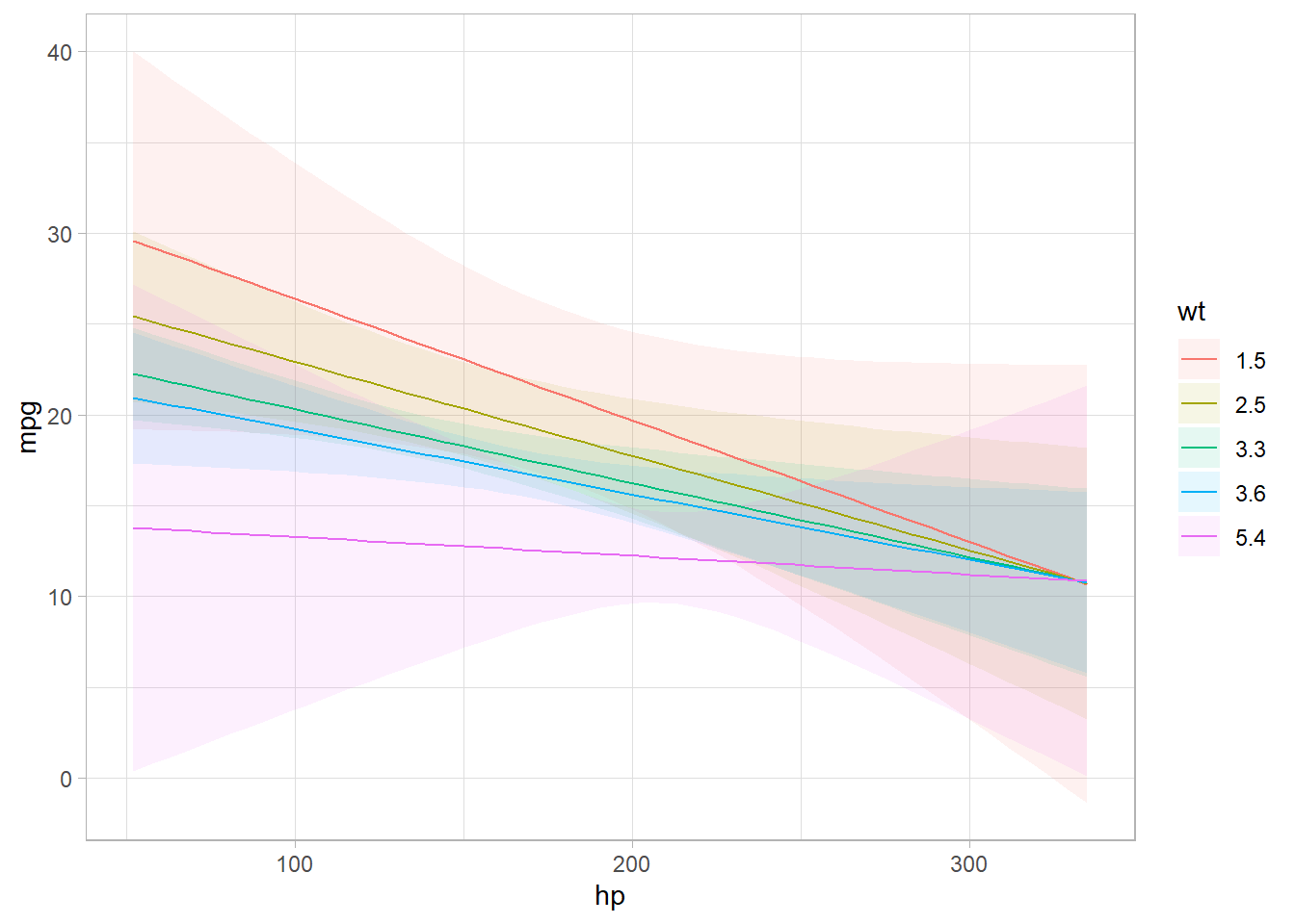
Figure 17.2: Line Chart Coefficients
Computing Marginal Effects
# Compute Average Marginal Effects (AME)
mfx <- marginaleffects::slopes(mod, variables = c("hp", "wt"))
head(mfx)
#>
#>  Estimate Std. Error     z Pr(>|z|)   S   2.5 %    97.5 %
#>   -0.0369     0.0185 -2.00  0.04598 4.4 -0.0732 -0.000659
#>   -0.0287     0.0156 -1.84  0.06630 3.9 -0.0593  0.001931
#>   -0.0466     0.0226 -2.06  0.03945 4.7 -0.0909 -0.002249
#>   -0.0423     0.0133 -3.18  0.00146 9.4 -0.0683 -0.016232
#>   -0.0390     0.0134 -2.91  0.00363 8.1 -0.0653 -0.012730
#>   -0.0387     0.0135 -2.87  0.00409 7.9 -0.0652 -0.012289
#>
#> Term: hp
#> Type: response
#> Comparison: dY/dX

# Compute Group-Average Marginal Effects
head(marginaleffects::slopes(mod, by = "hp", variables = "am"))
#>
#>  hp Estimate Std. Error      z Pr(>|z|)   S 2.5 % 97.5 %
#>  52     3.98       5.20  0.764    0.445 1.2 -6.22  14.18
#>  62    -2.77       2.51 -1.107    0.268 1.9 -7.68   2.14
#>  65     3.00       4.13  0.725    0.468 1.1 -5.10  11.10
#>  66     2.03       3.48  0.582    0.561 0.8 -4.80   8.85
#>  91     1.86       2.76  0.674    0.500 1.0 -3.54   7.26
#>  93     1.20       2.35  0.511    0.609 0.7 -3.40   5.80
#>
#> Term: am
#> Type: response
#> Comparison: 1 - 0

# Marginal Effects at Representative Values (MER)
marginaleffects::slopes(mod, newdata = datagrid(am = 0, wt = c(2, 4)))
#>
#>  Term Contrast am wt Estimate Std. Error      z Pr(>|z|)   S   2.5 %   97.5 %
#>    am    1 - 0  0  2   2.5474     2.7891  0.913   0.3611 1.5 -2.9191  8.01403
#>    am    1 - 0  0  4  -2.9541     3.0348 -0.973   0.3304 1.6 -8.9021  2.99400
#>    hp    dY/dX  0  2  -0.0598     0.0283 -2.115   0.0344 4.9 -0.1153 -0.00439
#>    hp    dY/dX  0  4  -0.0309     0.0187 -1.654   0.0982 3.3 -0.0676  0.00573
#>    wt    dY/dX  0  2  -2.6716     1.4149 -1.888   0.0590 4.1 -5.4449  0.10159
#>    wt    dY/dX  0  4  -2.6716     1.4154 -1.888   0.0591 4.1 -5.4458  0.10248
#>
#> Type: response

# Marginal Effects at the Mean (MEM)
marginaleffects::slopes(mod, newdata = "mean")
#>
#>  Term Contrast Estimate Std. Error      z Pr(>|z|)   S   2.5 %  97.5 %
#>    am    1 - 0  -0.8009     1.5219 -0.526  0.59871 0.7 -3.7837  2.1819
#>    hp    dY/dX  -0.0422     0.0133 -3.181  0.00147 9.4 -0.0683 -0.0162
#>    wt    dY/dX  -2.6716     1.4151 -1.888  0.05903 4.1 -5.4452  0.1019
#>
#> Type: response
Counterfactual Comparisons
# Counterfactual comparison: Effect of changing 'am' from 0 to 1
comparisons(mod, variables = list(am = 0:1))
#>
#>  Estimate Std. Error      z Pr(>|z|)   S 2.5 % 97.5 %
#>     0.325       1.68  0.193    0.847 0.2 -2.97   3.62
#>    -0.544       1.57 -0.347    0.729 0.5 -3.62   2.53
#>     1.201       2.35  0.511    0.609 0.7 -3.40   5.80
#>    -1.703       1.87 -0.912    0.362 1.5 -5.36   1.96
#>    -0.615       1.68 -0.366    0.715 0.5 -3.91   2.68
#> --- 22 rows omitted. See ?print.marginaleffects ---
#>     4.081       3.94  1.037    0.300 1.7 -3.63  11.79
#>     2.106       2.29  0.920    0.358 1.5 -2.38   6.59
#>     0.895       1.64  0.544    0.586 0.8 -2.33   4.12
#>     4.027       3.24  1.243    0.214 2.2 -2.32  10.38
#>    -0.237       1.59 -0.149    0.881 0.2 -3.35   2.87
#> Term: am
#> Type: response
#> Comparison: 1 - 0
17.7.2 margins Package
The margins package is a popular choice, designed to replicate Stata’s margins command in R. It provides marginal effects for each variable in a model, including interaction terms. margins define:
- Average Partial Effects: The contribution of each variable to the outcome scale, conditional on the other variables involved in the link function transformation of the linear predictor.
- Average Marginal Effects: The marginal contribution of each variable on the scale of the linear predictor.
- Average marginal effects represent the mean of these unit-specific partial derivatives over a given sample.
Key Features
Computes Average Partial Effects (APE).
Supports Marginal Effects at the Mean (MEM).
Provides visualizations of marginal effects.
Limitation:
- Slower than
marginaleffects, especially with large datasets.
library(margins)

# Fit a linear model with interactions
mod <- lm(mpg ~ cyl * hp + wt, data = mtcars)

# Compute marginal effects
summary(margins(mod))
#>  factor     AME     SE       z      p   lower   upper
#>     cyl  0.0381 0.5999  0.0636 0.9493 -1.1376  1.2139
#>      hp -0.0463 0.0145 -3.1909 0.0014 -0.0748 -0.0179
#>      wt -3.1198 0.6613 -4.7175 0.0000 -4.4160 -1.8236

# Equivalent function for summary
margins_summary(mod)
#>  factor     AME     SE       z      p   lower   upper
#>     cyl  0.0381 0.5999  0.0636 0.9493 -1.1376  1.2139
#>      hp -0.0463 0.0145 -3.1909 0.0014 -0.0748 -0.0179
#>      wt -3.1198 0.6613 -4.7175 0.0000 -4.4160 -1.8236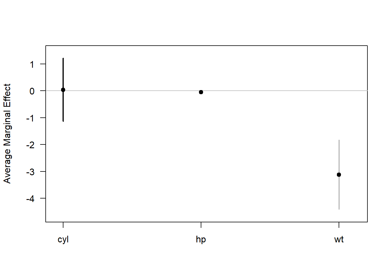
Figure 17.3: Average Marginal Effect
Marginal Effects at Representative Values
# Compute marginal effects when 'hp' = 150
margins(mod, at = list(hp = 150)) %>% summary()
#>  factor       hp     AME     SE       z      p   lower   upper
#>     cyl 150.0000  0.1009 0.6128  0.1647 0.8692 -1.1001  1.3019
#>      hp 150.0000 -0.0463 0.0145 -3.1909 0.0014 -0.0748 -0.0179
#>      wt 150.0000 -3.1198 0.6613 -4.7175 0.0000 -4.4160 -1.8236
17.7.3 mfx Package
The mfx package is specialized for GLMs, computing marginal effects for probit, logit, Poisson, and other count models.
Limitation:
- Computes only marginal effects for each variable, not the average marginal effect.
Supported Models in mfx
| Model | Outcome Type | Function |
|---|---|---|
| Probit | Binary | probitmfx() |
| Logit | Binary | logitmfx() |
| Poisson | Count | poissonmfx() |
| Negative Binomial | Count | negbinmfx() |
| Beta | Rate | betamfx() |
Example: Poisson Regression
library(mfx)
data("mtcars")

# Fit a Poisson model and compute marginal effects
poissonmfx(formula = vs ~ mpg * cyl * disp, data = mtcars)
#> Call:
#> poissonmfx(formula = vs ~ mpg * cyl * disp, data = mtcars)
#>
#> Marginal Effects:
#>                    dF/dx   Std. Err.       z  P>|z|
#> mpg           1.4722e-03  8.7531e-03  0.1682 0.8664
#> cyl           6.6420e-03  3.9263e-02  0.1692 0.8657
#> disp          1.5899e-04  9.4555e-04  0.1681 0.8665
#> mpg:cyl      -3.4698e-04  2.0564e-03 -0.1687 0.8660
#> mpg:disp     -7.6794e-06  4.5545e-05 -0.1686 0.8661
#> cyl:disp     -3.3837e-05  1.9919e-04 -0.1699 0.8651
#> mpg:cyl:disp  1.6812e-06  9.8919e-06  0.1700 0.8650
For more details, see the mfx vignette.
17.7.4 Comparison of Packages
| Feature |
marginaleffects (Recommended) |
margins |
mfx |
|---|---|---|---|
| Computes AME | Yes | Yes | No |
| Computes MEM | Yes | Yes | No |
| Computes MER | Yes | Yes | No |
| Supports GLM Models | Yes | Yes | Yes (but limited to glm) |
| Works with Interactions | Yes | Yes | No |
| Fast and Efficient | Yes | No (slower) | Yes (for GLMs) |
| Supports Counterfactuals | Yes | No | No |