44 High-Performance Computing

High-Performance Computing (HPC) refers to the use of advanced computational systems and techniques to solve complex, resource-intensive problems that are impractical or inefficient on standard computing platforms. In the realm of data analysis, HPC enables the handling of large-scale data processing, computationally intensive simulations, and advanced statistical modeling, particularly in fields like finance, marketing, bioinformatics, and engineering.

By leveraging parallel processing, either through multi-core processors on a single machine or distributed nodes in a computing cluster, HPC environments dramatically reduce execution times and expand analytical capabilities.

In the R programming ecosystem, several packages and frameworks facilitate parallel and distributed computing. These include:

parallel: Built-in R package for basic parallel operations.
foreach + doParallel: Enables parallel loops over independent tasks.
future: Provides a unified API for parallelization with different backends.
BiocParallel: Optimized for parallel evaluation in bioinformatics pipelines.
sparklyr: Connects R to Apache Spark for big data processing.
snow: For simpler parallel computing on Windows and Linux clusters.

However, effective HPC implementation requires more than just code parallelization. Testing, monitoring, estimating resource requirements, and iterative scaling are all essential components to maximize efficiency and prevent costly mistakes.

44.1 Best Practices for HPC in Data Analysis

Test First on a Small Scale

Before scaling your analysis to full production, begin with small-scale tests. This ensures your code runs as expected, while also providing crucial information about resource usage.

Start small: Run the analysis on a subset of your data (e.g., 1% or 10% of the total).
Measure resource usage:
- Execution time (wall clock time vs. CPU time).
- Memory footprint.
- CPU and disk I/O utilization.
Record the metrics:
- Create logs or structured reports for future reference.

Example:
If you’re modeling customer churn on a dataset of 10 million records, start with 100,000 and profile its behavior.

Estimate Resource Requirements

Use insights from small-scale tests to extrapolate the resources needed for the full analysis.

Estimate CPU cores, memory, and execution time requirements.
Add an overhead buffer:
- Parallel tasks introduce communication overhead and synchronization delays.
- Real-world data can have higher complexity than test data.

Guideline: If a small test consumes 1 GB of RAM and runs in 10 minutes on a single core, a 100x dataset may not scale linearly. Communication costs, disk I/O, and parallel inefficiencies could require a different scaling factor.

Parallelize Strategically

Not all parts of your analysis benefit equally from parallelization. Identify and prioritize computational bottlenecks.

Analyze your workflow:
- Data ingestion: Can you parallelize reading large files or querying databases?
- Transformations: Are data wrangling tasks parallelizable?
- Modeling/Training: Can independent model fits or simulations be distributed?
Balance granularity:
- Overly fine-grained parallelization leads to high communication overhead.
- Coarser tasks are generally more efficient in parallel environments.

Tip: Use embarrassingly parallel strategies where possible—these tasks require minimal communication between workers.

Use Adequate Scheduling and Queue Systems

In HPC clusters, job scheduling systems manage resource allocation and prioritize workloads.

Common systems include:

Slurm (Simple Linux Utility for Resource Management)
PBS (Portable Batch System)
LSF (Load Sharing Facility)
SGE (Sun Grid Engine)

Best practices:

Write job submission scripts specifying:
- Wall time limits.
- Memory and CPU requests.
- Node allocation (if required).
Monitor jobs:
- Examine logs for resource utilization (memory, time, CPU load).
- Use scheduler tools (e.g., sacct in Slurm) to assess historical performance.

Example Slurm job script:

#!/bin/bash
#SBATCH --job-name=churn_model
#SBATCH --output=churn_model_%j.out
#SBATCH --ntasks=1
#SBATCH --cpus-per-task=8
#SBATCH --mem=32G
#SBATCH --time=04:00:00

module load R/4.2.0
Rscript run_churn_model.R

Incremental Scaling

Resist the temptation to scale from small tests directly to massive production jobs.

Iterate gradually:
- Start with small jobs, progress to medium-sized runs, and only then scale to full production.
Monitor I/O overhead:
- Parallel jobs often stress shared storage systems.
- Optimize data locality and prefetching if possible.

Tip: Use asynchronous job submission (batchtools::submitJobs() or future::future()) to manage job batches efficiently.

Documentation and Reporting

Good documentation facilitates reproducibility and future optimization.

Maintain a structured report of each run, including:

Input parameters: Dataset size, preprocessing steps, model parameters.
Cluster specification: Number of nodes, CPUs per node, memory allocations.
Execution logs: Total run time, CPU utilization, memory usage.
Software environment: R version, package versions, job scheduler version.

Template for documentation:

Parameter	Value
Dataset size	10 million records
Model type	Random Forest (500 trees)
Nodes used	4
CPUs per node	8
Memory per node	32 GB
Wall time	2 hours
Software environment	R 4.2.0, ranger 0.14.1
Scheduler	Slurm 20.11.8

44.2 Example Workflow in R

Below is a conceptual R workflow demonstrating how to:

Load data and define a test subset.
Perform computations in parallel for the test subset using the parallel or foreach approach.
Measure resource usage (basic approach in R; for deeper HPC environment metrics, rely on the cluster’s job scheduler logs).
Extrapolate resource usage.
Submit a scaled-up job with new allocations.

44.3 Recommendations

Incremental Testing

Always begin with a small fraction of the data to validate your HPC pipeline and catch issues early.
Collect critical metrics:
- Run time (both wall clock time and CPU time).
- CPU utilization (are all requested cores working efficiently?).
- Memory usage (peak RAM consumption).
Use tools such as system.time(), profvis::profvis(), or Rprof() in R to profile your code locally before scaling.

Resource Allocation

Use test metrics to guide your resource requests (memory, cores, and wall time).
Avoid:
- Under-requesting: jobs may fail due to out-of-memory (OOM) errors or timeouts.
- Over-requesting: results in longer queue times, resource underutilization, and potential policy violations on shared systems.
Rule of thumb:
- Request slightly more memory than observed usage (e.g., 10-20% buffer).
- Request wall time based on observed run time, plus an additional safety margin (e.g., 15-30%).

Parallelization Strategy
- Identify tasks that can be embarrassingly parallel:
  - Monte Carlo simulations.
  - Bootstrap resampling.
  - Model fitting on independent data partitions.
- Focus on minimizing communication overhead:
  - Send only essential data between processes.
  - Use shared-memory parallelism when possible to avoid data duplication.
  - For distributed nodes, serialize and compress data before transmission when feasible.
Monitoring and Logging
- Use HPC job scheduler logs to track job performance:
  - Slurm: sacct, scontrol show job, or seff.
  - PBS/SGE: check standard output/error logs and resource summaries.
- Capture R logs and console output:
  - Direct output to log files using sink() or by redirecting standard output in your job script.
- Record:
  - Start and end times.
  - Memory and CPU metrics.
  - Warnings and error messages.
Scaling
- For large-scale runs (e.g., 100x your initial test), do not jump from small-scale to full-scale directly.
  - Run intermediate-scale tests (e.g., 10x, 50x).
  - Confirm resource usage scales as expected.
- Watch for non-linear effects:
  - Increased I/O overhead from parallel file reads/writes.
  - Communication overhead in distributed tasks.
  - Load balancing inefficiencies (stragglers can delay job completion).
Future-Proofing
- HPC hardware and software evolve rapidly:
  - Faster networks (InfiniBand, RDMA).
  - Improved schedulers and resource managers.
  - Containerization (Docker, Singularity) for reproducible environments.
- Regularly test and validate reproducibility after:
  - Software/package updates.
  - Hardware upgrades.
  - HPC policy changes (e.g., new quotas or job priorities).

44.4 Demonstration

###############################################################
# HPC Workflow Demo in R: Scaling Resources and Parallelism
###############################################################


# -- 1. Libraries --
library(parallel)       # base parallel
library(doParallel)     # foreach backend
library(foreach)        # parallel loops
library(future)         # futures
library(future.apply)   # apply with futures
library(ggplot2)        # plotting results

# Optional: install.packages("pryr") for memory usage (optional)
# library(pryr)

###############################################################
# -- 2. Generate or Load Data (Small and Large for Scaling) --
###############################################################

set.seed(42)

n_small <- 1e4    # Small dataset (test)
n_large <- 1e6    # Large dataset (scale-up demo)

generate_data <- function(n) {
    data.frame(
        id = 1:n,
        x = rnorm(n, mean = 50, sd = 10),
        y = rnorm(n, mean = 100, sd = 25)
    )
}

data_small <- generate_data(n_small)
data_large <- generate_data(n_large)

###############################################################
# -- 3. Preprocessing Function --
###############################################################

clean_and_transform <- function(df) {
    df$dist <- sqrt(df$x ^ 2 + df$y ^ 2)
    return(df)
}

data_small_clean <- clean_and_transform(data_small)
data_large_clean <- clean_and_transform(data_large)

###############################################################
# -- 4. Heavy Computation (Simulated Workload) --
###############################################################

heavy_computation <- function(df, reps = 500) {
    replicate(reps, sum(df$dist))
}

###############################################################
# -- 5. Resource Measurement Helper Function --
###############################################################

measure_resources <-
    function(expr, approach_name, data_size, cores) {
        start_time <- Sys.time()
        
        # baseline_mem <- pryr::mem_used()  # If pryr is available
        result <- eval(expr)
        end_time <- Sys.time()
        
        time_elapsed <-
            as.numeric(difftime(end_time, start_time, units = "secs"))
        # used_mem <- as.numeric(pryr::mem_used() - baseline_mem) / 1e6  # MB
        
        # If pryr isn't available, approximate:
        used_mem <- as.numeric(object.size(result)) / 1e6  # MB
        
        return(
            data.frame(
                Approach = approach_name,
                Data_Size = data_size,
                Cores = cores,
                Time_Sec = time_elapsed,
                Memory_MB = round(used_mem, 2)
            )
        )
    }

###############################################################
# -- 6. Define and Run Parallel Approaches --
###############################################################

# Collect results in a dataframe
results <- data.frame()

### 6.1 Single Core (Baseline)
res_single_small <- measure_resources(
    expr = quote(heavy_computation(data_small_clean)),
    approach_name = "SingleCore",
    data_size = nrow(data_small_clean),
    cores = 1
)

res_single_large <- measure_resources(
    expr = quote(heavy_computation(data_large_clean)),
    approach_name = "SingleCore",
    data_size = nrow(data_large_clean),
    cores = 1
)

results <- rbind(results, res_single_small, res_single_large)

# clusterExport(cl, varlist = c("heavy_computation"))


### 6.2 Base Parallel (Cross-Platform): parLapply (Cluster Based)
cores_to_test <- c(2, 4)

for (cores in cores_to_test) {
    cl <- makeCluster(cores)
    
    # Export both the heavy function and the datasets
    clusterExport(cl,
                  varlist = c(
                      "heavy_computation",
                      "data_small_clean",
                      "data_large_clean"
                  ))
    
    res_par_small <- measure_resources(
        expr = quote({
            parLapply(
                cl = cl,
                X = 1:cores,
                fun = function(i)
                    heavy_computation(data_small_clean)
            )
        }),
        approach_name = "parLapply",
        data_size = nrow(data_small_clean),
        cores = cores
    )
    
    res_par_large <- measure_resources(
        expr = quote({
            parLapply(
                cl = cl,
                X = 1:cores,
                fun = function(i)
                    heavy_computation(data_large_clean)
            )
        }),
        approach_name = "parLapply",
        data_size = nrow(data_large_clean),
        cores = cores
    )
    
    stopCluster(cl)
    
    results <- rbind(results, res_par_small, res_par_large)
}



### 6.3 foreach + doParallel
for (cores in cores_to_test) {
    cl <- makeCluster(cores)
    registerDoParallel(cl)
    
    clusterExport(cl,
                  varlist = c(
                      "heavy_computation",
                      "data_small_clean",
                      "data_large_clean"
                  ))
    registerDoParallel(cl)
    
    # Small dataset
    res_foreach_small <- measure_resources(
        expr = quote({
            foreach(i = 1:cores, .combine = c) %dopar% {
                heavy_computation(data_small_clean)
            }
        }),
        approach_name = "foreach_doParallel",
        data_size = nrow(data_small_clean),
        cores = cores
    )
    
    # Large dataset
    res_foreach_large <- measure_resources(
        expr = quote({
            foreach(i = 1:cores, .combine = c) %dopar% {
                heavy_computation(data_large_clean)
            }
        }),
        approach_name = "foreach_doParallel",
        data_size = nrow(data_large_clean),
        cores = cores
    )
    
    stopCluster(cl)
    
    results <- rbind(results, res_foreach_small, res_foreach_large)
}

### 6.4 future + future.apply
for (cores in cores_to_test) {
    plan(multicore, workers = cores)  # multicore only works on Unix; use multisession on Windows
    
    # Small dataset
    res_future_small <- measure_resources(
        expr = quote({
            future_lapply(1:cores, function(i)
                heavy_computation(data_small_clean))
        }),
        approach_name = "future_lapply",
        data_size = nrow(data_small_clean),
        cores = cores
    )
    
    # Large dataset
    res_future_large <- measure_resources(
        expr = quote({
            future_lapply(1:cores, function(i)
                heavy_computation(data_large_clean))
        }),
        approach_name = "future_lapply",
        data_size = nrow(data_large_clean),
        cores = cores
    )
    
    results <- rbind(results, res_future_small, res_future_large)
}

# Reset plan to sequential
plan(sequential)

###############################################################
# -- 7. Summarize and Plot Results --
###############################################################

# Print table
print(results)
#>              Approach Data_Size Cores   Time_Sec Memory_MB
#> 1          SingleCore     10000     1 0.01592588      0.00
#> 2          SingleCore   1000000     1 1.39803696      0.00
#> 3           parLapply     10000     2 0.01917386      0.01
#> 4           parLapply   1000000     2 1.39586711      0.01
#> 5           parLapply     10000     4 0.01869416      0.02
#> 6           parLapply   1000000     4 1.38051891      0.02
#> 7  foreach_doParallel     10000     2 0.05416512      0.01
#> 8  foreach_doParallel   1000000     2 1.39824295      0.01
#> 9  foreach_doParallel     10000     4 0.05402493      0.02
#> 10 foreach_doParallel   1000000     4 1.37731504      0.02
#> 11      future_lapply     10000     2 0.06894493      0.01
#> 12      future_lapply   1000000     2 2.96077895      0.01
#> 13      future_lapply     10000     4 0.09989095      0.02
#> 14      future_lapply   1000000     4 5.80409098      0.02

# Save to CSV
write.csv(results, "HPC_parallel_results.csv", row.names = FALSE)

# Plot Time vs. Data Size / Cores
ggplot(results, aes(x = as.factor(Cores), y = Time_Sec, fill = Approach)) +
    geom_bar(stat = "identity", position = "dodge") +
    facet_wrap( ~ Data_Size, scales = "free", labeller = label_both) +
    labs(title = "Runtime by Cores, Approach, and Data Size",
         x = "Number of Cores",
         y = "Time (Seconds)") +
    theme_minimal()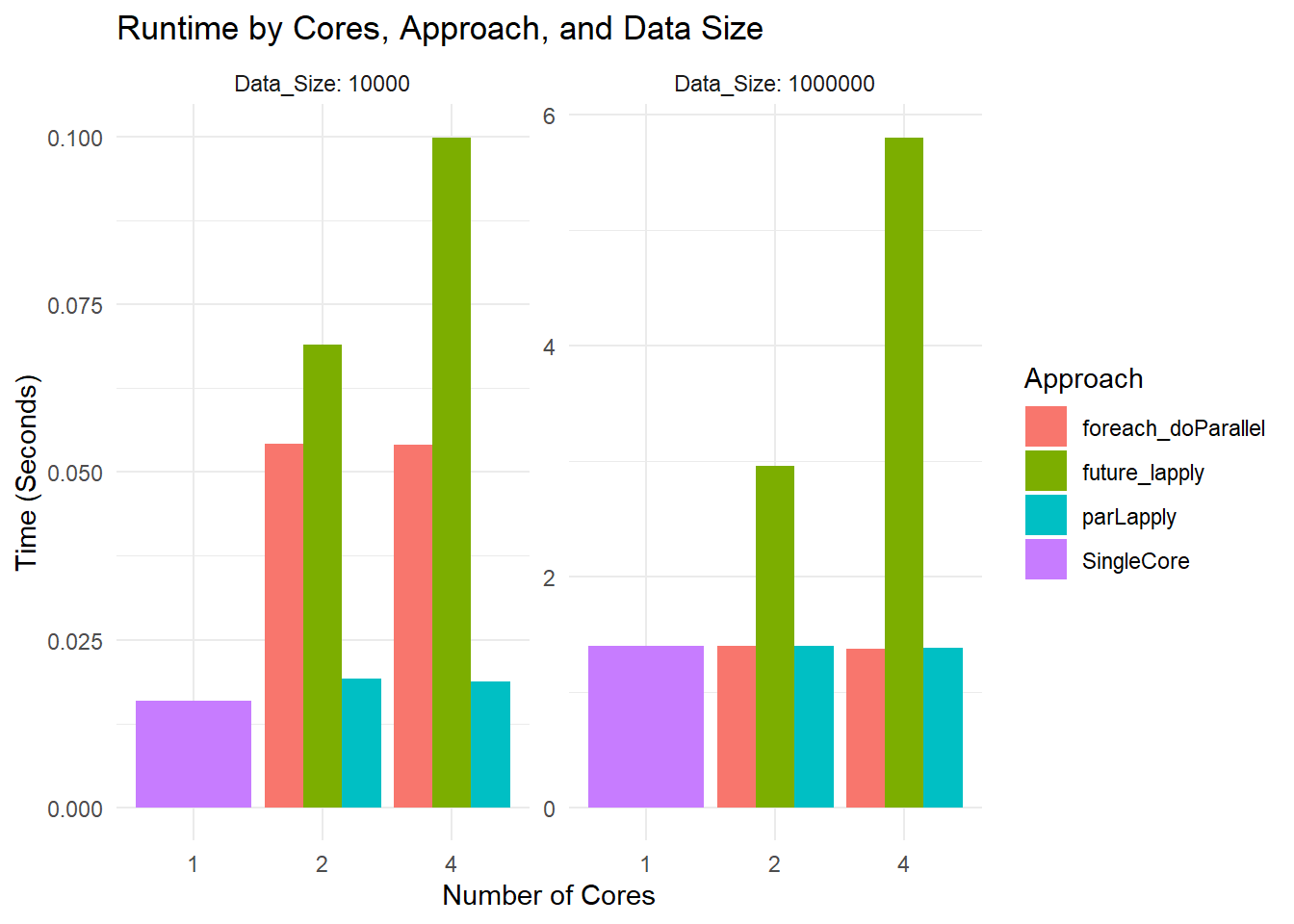


# Plot Memory Usage
ggplot(results, aes(x = as.factor(Cores), y = Memory_MB, fill = Approach)) +
    geom_bar(stat = "identity", position = "dodge") +
    facet_wrap(~ Data_Size, scales = "free", labeller = label_both) +
    labs(title = "Memory Usage by Cores, Approach, and Data Size",
         x = "Number of Cores",
         y = "Memory (MB)") +
    theme_minimal()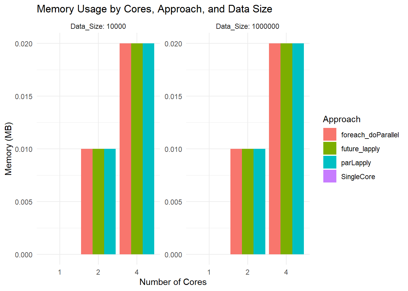

Runtime Plot
- Small Dataset: All methods are so fast that you are mostly seeing overhead differences. The differences in bar heights reflect how each parallel framework handles overhead.
- Large Dataset: You see more separation. For instance, parLapply with 2 cores might be slower than 1 core due to overhead. At 4 cores, it might improve or not, depending on how the overhead and actual workload balance out.
Memory Usage Plot
- All bars hover around 0.02 MB or so because you are measuring the size of the returned result, not the in-memory size of the large dataset. The function object.size(result) is not capturing total RAM usage by the entire parallel job.

43 Replication and Synthetic Data

A Appendix