29 Synthetic Difference-in-Differences
Understanding the impact of policy interventions is a fundamental challenge in empirical research. Analysts frequently rely on panel data, which tracks multiple units over time, to assess how outcomes change before and after a policy is implemented. However, estimating causal effects in this setting is complicated by the fact that policies are often adopted non-randomly, where certain units may be more likely to receive treatment based on their characteristics, prior trends, or external factors. If treatment assignment correlates with unit-specific or time-specific factors, selection bias can invalidate causal conclusions, even when observed covariates are accounted for (G. W. Imbens and Rubin 2015).
A well-established approach to dealing with this challenge is the Difference-in-Differences (DID) method, which compares changes in outcomes between treated and untreated groups. However, DID relies on the crucial parallel trends assumption (the idea that, in the absence of treatment, treated and untreated units would have followed similar trajectories). When this assumption is violated, DID can produce biased estimates.
An alternative approach, Synthetic Control (SC), is particularly useful when only a few units receive treatment. Instead of assuming parallel trends, SC constructs a weighted combination of untreated units that best approximates the pre-treatment behavior of the treated group. This method improves comparability but has limitations, including sensitivity to extrapolation and instability when there are many control units.
To address the shortcomings of both DID and SC, Synthetic Difference-in-Differences (SDID) was introduced by Arkhangelsky et al. (2021). SDID is a weighted double-differencing estimator that:
- Combines features of DID and SC to improve causal inference.
- Adjusts for differences in pre-treatment trends through reweighting (like SC).
- Remains invariant to additive unit-level shifts and is valid for large panels (like DID).
The key advantage of SDID is that it achieves double robustness: it performs well when DID assumptions hold but also corrects for deviations from parallel trends by using synthetic weights (Table 29.1). This makes SDID particularly useful in situations where treatment assignment is correlated with latent factors that affect outcomes over time.
- SDID explicitly accounts for systematic unit-level effects that influence treatment assignment.
- This is especially valuable when treatment is non-randomly assigned based on persistent unit characteristics.
- Even under purely random treatment assignment, all three methods (DID, SC, and SDID) are unbiased, but SDID achieves the smallest standard errors.
Recent research has applied SDID to evaluate marketing interventions and policy changes:
- TV Advertising & Online Sales (Lambrecht, Tucker, and Zhang 2024): SDID was used to estimate the effect of TV ad campaigns on consumer behavior, accounting for time-varying confounders.
- Soda Tax & Marketing Effectiveness (Keller, Guyt, and Grewal 2024): SDID helped measure how soda tax policies influenced marketing strategies and consumer demand.
| Method | Assumptions | Use Case | Strengths | Weaknesses |
|---|---|---|---|---|
| DID | Parallel trends assumption | Many treated units | Simple implementation, valid for large panels | Fails when parallel trends assumption is violated |
| SC | Reweighting to match pre-treatment trends | Few treated units | More flexible, compensates for lack of parallel trends | Sensitive to outliers, does not scale well with large treated groups |
Attractive Features of SDID
-
Statistical Properties
- Provides consistent and asymptotically normal estimates.
- Achieves double robustness, similar to augmented inverse probability weighting estimators Scharfstein, Rotnitzky, and Robins (1999).
-
Performance Comparison
- In settings where DID is valid, SDID performs at least as well or better.
- Unlike DID, SDID remains valid when treatment assignment correlates with latent unit-level or time-varying factors.
- In settings where SC is used, SDID performs equally well or better.
- When treatment is randomly assigned, all methods remain unbiased, but SDID tends to have higher precision.
- Bias Reduction
-
Related to Augmented SC
- Shares methodological similarities with augmented SC estimators (Ben-Michael, Feller, and Rothstein 2021; Arkhangelsky et al. 2021, 4112).
-
Recommended Use Cases
SDID is particularly effective when:- The number of control units (\(N_{ctr}\)) is similar to the number of pre-treatment periods (\(T_{pre}\)).
- The number of post-treatment periods (\(T_{post}\)) is small.
- The number of treated units (\(N_{tr}\)) satisfies:
\[ N_{tr} < \sqrt{N_{ctr}} \]
29.1 Understanding
To formally define the SDID estimator, we begin by considering a balanced panel dataset with \(N\) units observed over \(T\) time periods. Our goal is to estimate the causal effect of a treatment intervention while accounting for both unit-specific and time-specific confounders.
Let:
- \(Y_{it}\) be the outcome variable for unit \(i\) at time \(t\).
- \(W_{it} \in \{0,1\}\) be a binary indicator of treatment, where \(W_{it} = 1\) if unit \(i\) is treated at time \(t\) and \(0\) otherwise.
- The panel consists of:
- \(N_c\) control units (never treated).
- \(N_t\) treated units, exposed to treatment after period \(T_{pre}\).
29.1.1 Steps in SDID Estimation
SDID combines ideas from both SC and DID by introducing unit weights and time weights:
Find unit weights \(\hat{w}_i^{sdid}\) to ensure that pre-treatment outcomes of the weighted control group match the pre-treatment outcomes of the treated units:
\[ \sum_{i = 1}^{N_c} \hat{w}_i^{sdid} Y_{it} \approx \frac{1}{N_t} \sum_{i = N_c + 1}^{N} Y_{it}, \quad \forall t = 1, \dots, T_{pre} \]
This ensures that pre-treatment trends of treated and control units are similar, just as in SC.Find time weights \(\hat{\lambda}_t^{sdid}\) to balance post-treatment deviations from pre-treatment outcomes, stabilizing the inference.
-
Estimate the treatment effect \(\hat{\tau}^{sdid}\) by solving the following minimization problem:
\[ (\hat{\tau}^{sdid}, \hat{\mu}, \hat{\alpha}, \hat{\beta}) = \arg \min_{\tau, \mu, \alpha, \beta} \sum_{i=1}^{N} \sum_{t=1}^{T} (Y_{it} - \mu - \alpha_i - \beta_t - W_{it} \tau)^2 \hat{w}_i^{sdid} \hat{\lambda}_t^{sdid} \]
where:- \(\mu\) is the global intercept.
- \(\alpha_i\) captures unit-specific fixed effects.
- \(\beta_t\) captures time-specific fixed effects.
- \(\tau\) represents the treatment effect.
Unlike the standard DID and SC estimators, SDID incorporates both unit and time weights, making it less sensitive to violations of parallel trends.
DID solves:
\[
(\hat{\tau}^{did}, \hat{\mu}, \hat{\alpha}, \hat{\beta}) = \arg \min_{\tau, \mu, \alpha, \beta} \sum_{i=1}^{N} \sum_{t=1}^{T} (Y_{it} - \mu - \alpha_i - \beta_t - W_{it} \tau)^2
\]
However, DID does not use unit or time weights, making it unreliable if treatment assignment correlates with unobserved factors.
SC minimizes:
\[
(\hat{\tau}^{sc}, \hat{\mu}, \hat{\beta}) = \arg \min_{\tau, \mu, \beta} \sum_{i=1}^{N} \sum_{t=1}^{T} (Y_{it} - \mu - \beta_t - W_{it} \tau)^2 \hat{w}_i^{sdid}
\]
SC does not include unit fixed effects (\(\alpha_i\)) or time weights (\(\hat{\lambda}_t\)), which can introduce bias when unmeasured confounders vary over time.
29.1.2 Comparison of Methods
Table 29.2 summarizes key differences between DID, SC, and SDID:
| DID | SC | SDID | |
|---|---|---|---|
| Primary Assumption | Absence of intervention leads to parallel evolution across states. | Reweights unexposed states to match pre-intervention outcomes of treated state. | Reweights control units to ensure a parallel time trend with the treated pre-intervention trend. |
| Reliability Concern | Can be unreliable when pre-intervention trends aren’t parallel. | Accounts for non-parallel pre-intervention trends by reweighting. | Uses reweighting to adjust for non-parallel pre-intervention trends. |
| Treatment of Time Periods | All pre-treatment periods are given equal weight. | Doesn’t specifically emphasize equal weight for pre-treatment periods. | Focuses only on a subset of pre-intervention time periods, selected based on historical outcomes. |
| Goal with Reweighting | N/A (doesn’t use reweighting). | To match treated state as closely as possible before the intervention. | Make trends of control units parallel (not necessarily identical) to the treated pre-intervention. |
An alternative formulation of the SDID treatment effect is:
\[
\hat{\tau} = \hat{\delta}_t - \sum_{i = 1}^{N_c} \hat{w}_i^{sdid} \hat{\delta}_i
\]
where:
- \(\hat{\delta}_t = \frac{1}{N_t} \sum_{i = N_c + 1}^{N} \hat{\delta}_i\) represents the average deviation in treated units post-treatment (Table 29.3).
- \(\sum_{i = 1}^{N_c} \hat{w}_i^{sdid} \hat{\delta}_i\) adjusts for differences using weighted control unit deviations.
| Method | Sample Weight | Adjusted outcomes (\(\hat{\delta}_i\)) | Interpretation |
|---|---|---|---|
| SC | \(\hat{w}^{sc} = \min_{w \in R}l_{unit}(w)\) | \(\frac{1}{T_{post}} \sum_{t = T_{pre} + 1}^T Y_{it}\) | Unweighted treatment period averages |
| DID | \(\hat{w}_i^{did} = N_c^{-1}\) | \(\frac{1}{T_{post}} \sum_{t = T_{pre}+ 1}^T Y_{it} - \frac{1}{T_{pre}} \sum_{t = 1}^{T_{pre}}Y_{it}\) | Unweighted differences between average treatment period and pretreatment outcome |
| SDID | \((\hat{w}_0, \hat{w}^{sdid}) = \min l_{unit}(w_0, w)\) | \(\frac{1}{T_{post}} \sum_{t = T_{pre} + 1}^T Y_{it} - \sum_{t = 1}^{T_{pre}} \hat{\lambda}_t^{sdid} Y_{it}\) | Weighted differences between average treatment period and pretreatment outcome |
A key innovation in Synthetic Difference-in-Differences is its use of unit and time weights to refine causal estimates. By applying weights, SDID essentially localizes a standard two-way fixed effects regression, making it more robust and precise.
29.1.3 Why Use Weights?
- Unit weights (\(\hat{w}_i^{sdid}\)) emphasize control units that are most similar to the treated units based on pre-treatment trends.
- Time weights (\(\hat{\lambda}_t^{sdid}\)) prioritize time periods most comparable to the post-treatment period.
- This approach improves parallel trends validity without requiring a perfect match in raw data.
29.1.4 Benefits of Localization in SDID
-
Robustness
- By focusing on comparable units and time periods, SDID reduces bias from dissimilar observations.
- Improved Precision
29.1.5 Designing SDID Weights
29.1.5.1 Unit Weights: Balancing Pre-Treatment Trends
Unit weights \(\hat{w}_i^{sdid}\) ensure that the weighted control group mimics the treated group’s pre-treatment trends, similar to SC but with greater flexibility:
\[
\sum_{i = 1}^{N_c} \hat{w}_i^{sdid} Y_{it} \approx \frac{1}{N_t} \sum_{i = N_c + 1}^{N} Y_{it}, \quad \forall t = 1, \dots, T_{pre}
\]
This helps achieve parallel pre-treatment trends rather than requiring an exact match in levels.
29.1.5.2 Time Weights: Stabilizing Post-Treatment Inference
Time weights \(\hat{\lambda}_t^{sdid}\) ensure that post-treatment deviations are balanced relative to pre-treatment trends. This minimizes bias by down-weighting time periods that are vastly different from the post-treatment period.
- Unlike unit weights, time weights do not require regularization because outcomes within the same time period are highly correlated across units.
- Time weights improve the precision of SDID estimates by preventing certain periods from dominating the estimation process.
29.1.6 How SDID Enhances DID’s Plausibility
DID assumes parallel trends, but raw data often violates this assumption. SDID corrects for non-parallel trends by weighting both units and time periods.
- Similar techniques have been used before to adjust DID assumptions, such as controlling for covariates or selecting specific time periods (Callaway and Sant’Anna 2021).
- SDID automates this process, applying a systematic weighting approach for both units and time periods.
Including unit fixed effects (\(\alpha_i\)) in SDID has two main advantages:
-
Flexibility:
- Allows for systematic differences across units while preserving parallel trends after reweighting.
-
Enhanced Precision:
- Explains a large fraction of the variation in outcomes, reducing noise and improving estimation accuracy.
Unit Fixed Effects and SC Weighting
- Under ideal conditions, SC reweighting alone could account for unit fixed effects, if the weighted average of control unit outcomes perfectly matched the treated unit’s pre-treatment trajectory.
- However, this rarely happens in reality, making unit fixed effects necessary for robust inference.
- The use of fixed effects in synthetic control regressions (SC with intercept) was first proposed in Doudchenko and Imbens (2016) and Ferman and Pinto (2021), where it was referred to as DIFP (Difference-in-Fixed-Effects Prediction).
29.1.7 Choosing SDID Weights
- Choosing Unit Weights
Regularization Parameter:
- The penalty term is calibrated based on the typical one-period change in control unit outcomes during the pre-treatment period.
- This value is then multiplied by a scaling factor (Arkhangelsky et al. 2021, 4092).
Relation to Synthetic Control Weights:
SDID weights resemble those used in Abadie, Diamond, and Hainmueller (2010) but have two key modifications:
-
Inclusion of an Intercept Term
- Unlike SC, SDID does not force the control pre-trends to exactly match the treated pre-trends. Iit only ensures they are parallel.
- This flexibility arises from unit fixed effects, which absorb any systematic level differences.
-
Regularization Penalty
- Borrowed from Doudchenko and Imbens (2016).
- Ensures dispersion of weights, preventing over-reliance on a few control units.
- This guarantees a unique solution for unit weights.
How SDID Compares to DID Weights:
- DID weights are a special case of SC weights without an intercept or regularization penalty.
- DID applies unit weights as in SC but only when there is one treated unit.
- Choosing Time Weights
- Like unit weights, time weights include an intercept term to account for overall time effects.
- No regularization is applied to time weights because within-period correlations across units are expected.
- This design allows SDID to minimize bias while stabilizing inference.
29.1.8 Accounting for Time-Varying Covariates in Weight Estimation
To further refine the estimation process, SDID can incorporate time-varying covariates by adjusting the outcome variable:
\[ Y_{it}^{res} = Y_{it} - X_{it} \hat{\beta} \]
where \(\hat{\beta}\) comes from the regression:
\[ Y_{it} = X_{it} \beta + \varepsilon_{it} \]
This residualized outcome (\(Y_{it}^{res}\)) ensures that the weighting process accounts for time-varying confounders, improving the validity of causal estimates.
29.2 Application
SDID Algorithm
- Compute regularization parameter \(\zeta\)
\[ \zeta = (N_{t}T_{post})^{1/4} \hat{\sigma} \]
where
\[ \hat{\sigma}^2 = \frac{1}{N_c(T_{pre}- 1)} \sum_{i = 1}^{N_c} \sum_{t = 1}^{T_{re}-1}(\Delta_{it} - \hat{\Delta})^2 \]
\(\Delta_{it} = Y_{i(t + 1)} - Y_{it}\)
\(\hat{\Delta} = \frac{1}{N_c(T_{pre} - 1)}\sum_{i = 1}^{N_c}\sum_{t = 1}^{T_{pre}-1} \Delta_{it}\)
- Compute unit weights \(\hat{w}^{sdid}\)
\[ (\hat{w}_0, \hat{w}^{sidid}) = \arg \min_{w_0 \in R, w \in \Omega}l_{unit}(w_0, w) \]
where
\(l_{unit} (w_0, w) = \sum_{t = 1}^{T_{pre}}(w_0 + \sum_{i = 1}^{N_c}w_i Y_{it} - \frac{1}{N_t}\sum_{i = N_c + 1}^NY_{it})^2 + \zeta^2 T_{pre}||w||_2^2\)
\(\Omega = \{w \in R_+^N: \sum_{i = 1}^{N_c} w_i = 1, w_i = N_t^{-1} \forall i = N_c + 1, \dots, N \}\)
- Compute time weights \(\hat{\lambda}^{sdid}\)
\[ (\hat{\lambda}_0 , \hat{\lambda}^{sdid}) = \arg \min_{\lambda_0 \in R, \lambda \in \Lambda} l_{time}(\lambda_0, \lambda) \]
where
\(l_{time} (\lambda_0, \lambda) = \sum_{i = 1}^{N_c}(\lambda_0 + \sum_{t = 1}^{T_{pre}} \lambda_t Y_{it} - \frac{1}{T_{post}} \sum_{t = T_{pre} + 1}^T Y_{it})^2\)
\(\Lambda = \{ \lambda \in R_+^T: \sum_{t = 1}^{T_{pre}} \lambda_t = 1, \lambda_t = T_{post}^{-1} \forall t = T_{pre} + 1, \dots, T\}\)
- Compute the SDID estimator
\[ (\hat{\tau}^{sdid}, \hat{\mu}, \hat{\alpha}, \hat{\beta}) = \arg \min_{\tau, \mu, \alpha, \beta}\{ \sum_{i = 1}^N \sum_{t = 1}^T (Y_{it} - \mu - \alpha_i - \beta_t - W_{it} \tau)^2 \hat{w}_i^{sdid}\hat{\lambda}_t^{sdid} \]
SE Estimation
Under certain assumptions (errors, samples, and interaction properties between time and unit fixed effects) detailed in (Arkhangelsky et al. 2019, 4107), SDID is asymptotically normal and zero-centered
Using its asymptotic variance, conventional confidence intervals can be applied to SDID.
\[ \tau \in \hat{\tau}^{sdid} \pm z_{\alpha/2}\sqrt{\hat{V}_\tau} \]
-
There are 3 approaches for variance estimation in confidence intervals:
-
Clustered Bootstrap (Efron 1992):
Independently resample units.
Advantages: Simple to use; robust performance in large panels due to natural approach to inference with panel data where observations of the same unit might be correlated.
Disadvantage: Computationally expensive.
-
Jackknife (Miller 1974):
Applied to weighted SDID regression with fixed weights.
Generally conservative and precise when treated and control units are sufficiently similar.
Not recommended for some methods, like the SC estimator, due to potential biases.
Appropriate for jackknifing DID without random weights.
-
Placebo Variance Estimation:
Can used in cases with only one treated unit or large panels.
Placebo evaluations swap out the treated unit for untreated ones to estimate noise.
Relies on homoskedasticity across units.
Depends on homoskedasticity across units. It hinges on the empirical distribution of residuals from placebo estimators on control units.
The validity of the placebo method hinges on consistent noise distribution across units. One treated unit makes nonparametric variance estimation difficult, necessitating homoskedasticity for feasible inference. Detailed analysis available in Conley and Taber (2011).
-
All algorithms are from Arkhangelsky et al. (2021), p. 4109:
Bootstrap Variance Estimation
For each \(b\) from \(1 \to B\):
Sample \(N\) rows from \((\mathbf{Y}, \mathbf{W})\) to get (\(\mathbf{Y}^{(b)}, \mathbf{W}^{(b)}\)) with replacement.
If the sample lacks treated or control units, resample.
Calculate \(\tau^{(b)}\) using (\(\mathbf{Y}^{(b)}, \mathbf{W}^{(b)}\)).
Calculate variance: \(\hat{V}_\tau = \frac{1}{B} \sum_{b = 1}^B (\hat{\tau}^{b} - \frac{1}{B} \sum_{b = 1}^B \hat{\tau}^b)^2\)
Jackknife Variance Estimation
- For each \(i\) from \(1 \to N\):
- Calculate \(\hat{\tau}^{(-i)}\): \(\arg\min_{\tau, \{\alpha_j, \beta_t\}} \sum_{j \neq, i, t}(\mathbf{Y}_{jt} - \alpha_j - \beta_t - \tau \mathbf{W}_{it})^2 \hat{w}_j \hat{\lambda}_t\)
- Calculate: \(\hat{V}_{\tau} = (N - 1) N^{-1} \sum_{i = 1}^N (\hat{\tau}^{(-i)} - \hat{\tau})^2\)
Placebo Variance Estimation
- For each \(b\) from \(1 \to B\)
- Sample \(N_t\) out of \(N_c\) without replacement to get the “placebo” treatment
- Construct a placebo treatment matrix \(\mathbf{W}_c^b\) for the controls
- Calculate \(\hat{\tau}\) based on \((\mathbf{Y}_c, \mathbf{W}_c^b)\)
- Calculate \(\hat{V}_\tau = \frac{1}{B}\sum_{b = 1}^B (\hat{\tau}^b - \frac{1}{B} \sum_{b = 1}^B \hat{\tau}^b)^2\)
29.2.1 Block Treatment
Code provided by the synthdid package
library(synthdid)
library(tidyverse)

# Estimate the effect of California Proposition 99 on cigarette consumption
data('california_prop99')

setup = synthdid::panel.matrices(synthdid::california_prop99)

tau.hat = synthdid::synthdid_estimate(setup$Y, setup$N0, setup$T0)

# se = sqrt(vcov(tau.hat, method = 'placebo'))
Figure 29.1 shows the trajectories between treated units and synthetic control counterfactual units.
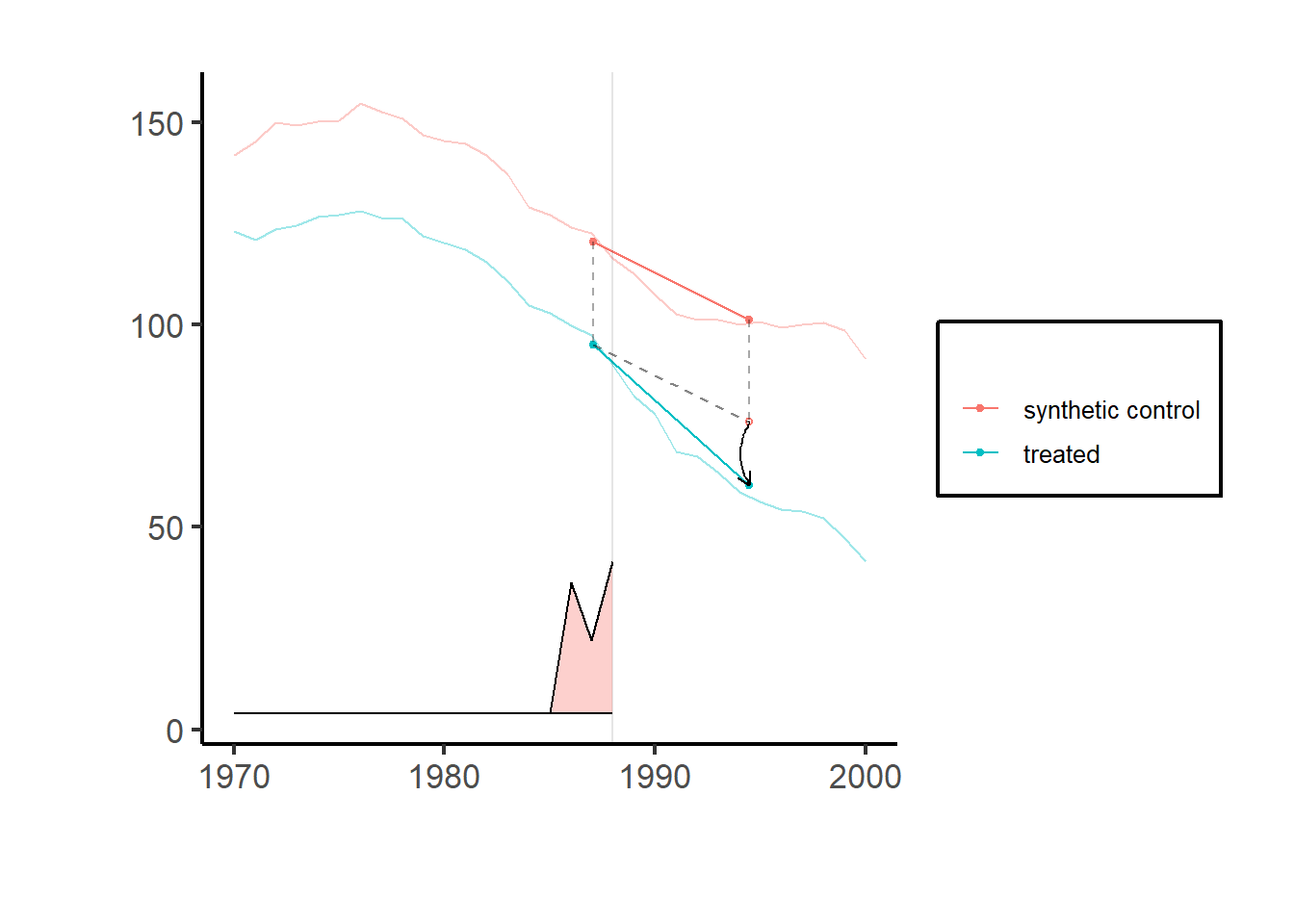
Figure 29.1: Synthetic Control Method: Treated vs. Synthetic Counterfactual Over Time
setup = synthdid::panel.matrices(synthdid::california_prop99)

# Run for specific estimators
results_selected = causalverse::panel_estimate(setup,
                                               selected_estimators = c("synthdid", "did", "sc"))

results_selected
#> $synthdid
#> $synthdid$estimate
#> synthdid: -15.604 +- NA. Effective N0/N0 = 16.4/38~0.4. Effective T0/T0 = 2.8/19~0.1. N1,T1 = 1,12.
#>
#> $synthdid$std.error
#> [1] 10.05324
#>
#>
#> $did
#> $did$estimate
#> synthdid: -27.349 +- NA. Effective N0/N0 = 38.0/38~1.0. Effective T0/T0 = 19.0/19~1.0. N1,T1 = 1,12.
#>
#> $did$std.error
#> [1] 15.81479
#>
#>
#> $sc
#> $sc$estimate
#> synthdid: -19.620 +- NA. Effective N0/N0 = 3.8/38~0.1. Effective T0/T0 = Inf/19~Inf. N1,T1 = 1,12.
#>
#> $sc$std.error
#> [1] 11.16422

# to access more details in the estimate object
summary(results_selected$did$estimate)
#> $estimate
#> [1] -27.34911
#>
#> $se
#>      [,1]
#> [1,]   NA
#>
#> $controls
#>                estimate 1
#> Wyoming             0.026
#> Wisconsin           0.026
#> West Virginia       0.026
#> Virginia            0.026
#> Vermont             0.026
#> Utah                0.026
#> Texas               0.026
#> Tennessee           0.026
#> South Dakota        0.026
#> South Carolina      0.026
#> Rhode Island        0.026
#> Pennsylvania        0.026
#> Oklahoma            0.026
#> Ohio                0.026
#> North Dakota        0.026
#> North Carolina      0.026
#> New Mexico          0.026
#> New Hampshire       0.026
#> Nevada              0.026
#> Nebraska            0.026
#> Montana             0.026
#> Missouri            0.026
#> Mississippi         0.026
#> Minnesota           0.026
#> Maine               0.026
#> Louisiana           0.026
#> Kentucky            0.026
#> Kansas              0.026
#> Iowa                0.026
#> Indiana             0.026
#> Illinois            0.026
#> Idaho               0.026
#> Georgia             0.026
#> Delaware            0.026
#> Connecticut         0.026
#>
#> $periods
#>      estimate 1
#> 1988      0.053
#> 1987      0.053
#> 1986      0.053
#> 1985      0.053
#> 1984      0.053
#> 1983      0.053
#> 1982      0.053
#> 1981      0.053
#> 1980      0.053
#> 1979      0.053
#> 1978      0.053
#> 1977      0.053
#> 1976      0.053
#> 1975      0.053
#> 1974      0.053
#> 1973      0.053
#> 1972      0.053
#> 1971      0.053
#>
#> $dimensions
#>           N1           N0 N0.effective           T1           T0 T0.effective
#>            1           38           38           12           19           19

causalverse::process_panel_estimate(results_selected)
#>     Method Estimate    SE
#> 1 SYNTHDID   -15.60 10.05
#> 2      DID   -27.35 15.81
#> 3       SC   -19.62 11.16
29.2.2 Staggered Adoption
To apply to staggered adoption settings using the SDID estimator (see examples in Arkhangelsky et al. (2021), p. 4115 similar to Ben-Michael, Feller, and Rothstein (2022)), we can:
Apply the SDID estimator repeatedly, once for every adoption date.
Using Ben-Michael, Feller, and Rothstein (2022) ’s method, form matrices for each adoption date. Apply SDID and average based on treated unit/time-period fractions.
Create multiple samples by splitting the data up by time periods. Each sample should have a consistent adoption date.
For a formal note on this special case, see Porreca (2022). It compares the outcomes from using SynthDiD with those from other estimators:
Two-Way Fixed Effects (TWFE),
The group time average treatment effect estimator from Callaway and Sant’Anna (2021),
The partially pooled synthetic control method estimator from Ben-Michael, Feller, and Rothstein (2021), in a staggered treatment adoption context.
-
The findings reveal that SynthDiD produces a different estimate of the average treatment effect compared to the other methods.
- Simulation results suggest that these differences could be due to the SynthDiD’s data generating process assumption (a latent factor model) aligning more closely with the actual data than the additive fixed effects model assumed by traditional DiD methods.
To explore heterogeneity of treatment effect, we can do subgroup analysis (Berman and Israeli 2022, 1092). Table 29.4 shows ways to perform valid subgroup analysis.
| Method | Advantages | Disadvantages | Procedure |
|---|---|---|---|
| Split Data into Subsets | Compares treated units to control units within the same subgroup. | Each subset uses a different synthetic control, making it challenging to compare effects across subgroups. |
|
| Control Group Comprising All Non-adopters | Control weights match pretrends well for each treated subgroup. | Each control unit receives a different weight for each treatment subgroup, making it difficult to compare results due to varying synthetic controls. |
|
| Use All Data to Estimate Synthetic Control Weights (recommend) | All units have the same synthetic control. | Pretrend match may not be as accurate since it aims to match the average outcome of all treated units, not just a specific subgroup. |
|
library(tidyverse)
df <- fixest::base_stagg |>
   dplyr::mutate(treatvar = if_else(time_to_treatment >= 0, 1, 0)) |>
   dplyr::mutate(treatvar = as.integer(if_else(year_treated > (5 + 2), 0, treatvar)))


est <- causalverse::synthdid_est_ate(
  data               = df,
  adoption_cohorts   = 5:7,
  lags               = 2,
  leads              = 2,
  time_var           = "year",
  unit_id_var        = "id",
  treated_period_var = "year_treated",
  treat_stat_var     = "treatvar",
  outcome_var        = "y"
)
#> Adoption Cohort: 5
#> Treated units: 5 Control units: 65
#> Adoption Cohort: 6
#> Treated units: 5 Control units: 60
#> Adoption Cohort: 7
#> Treated units: 5 Control units: 55

data.frame(
    Period = names(est$TE_mean_w),
    ATE    = est$TE_mean_w,
    SE     = est$SE_mean_w
) |>
    causalverse::nice_tab()
#>    Period   ATE   SE
#> 1      -2 -0.05 0.22
#> 2      -1  0.05 0.22
#> 3       0 -5.07 0.80
#> 4       1 -4.68 0.51
#> 5       2 -3.70 0.79
#> 6 cumul.0 -5.07 0.80
#> 7 cumul.1 -4.87 0.55
#> 8 cumul.2 -4.48 0.53
Figure 29.2 shows the average treatment effect over time.
causalverse::synthdid_plot_ate(est)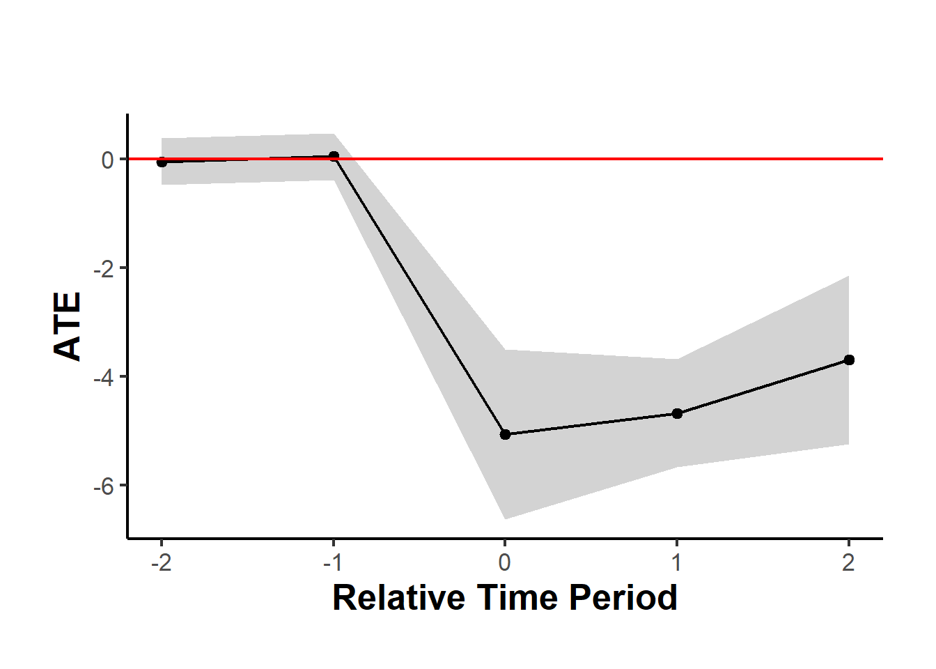
Figure 29.2: Event Study Plot of Average Treatment Effect Over Time
est_sub <- causalverse::synthdid_est_ate(
  data               = df,
  adoption_cohorts   = 5:7,
  lags               = 2,
  leads              = 2,
  time_var           = "year",
  unit_id_var        = "id",
  treated_period_var = "year_treated",
  treat_stat_var     = "treatvar",
  outcome_var        = "y",
  # a vector of subgroup id (from unit id)
  subgroup           =  c(
    # some are treated
    "11", "30", "49" ,
    # some are control within this period
    "20", "25", "21")
)
#> Adoption Cohort: 5
#> Treated units: 3 Control units: 65
#> Adoption Cohort: 6
#> Treated units: 0 Control units: 60
#> Adoption Cohort: 7
#> Treated units: 0 Control units: 55

data.frame(
    Period = names(est_sub$TE_mean_w),
    ATE = est_sub$TE_mean_w,
    SE = est_sub$SE_mean_w
) |>
    causalverse::nice_tab()
#>    Period   ATE   SE
#> 1      -2  0.32 0.44
#> 2      -1 -0.32 0.44
#> 3       0 -4.29 1.68
#> 4       1 -4.00 1.52
#> 5       2 -3.44 2.90
#> 6 cumul.0 -4.29 1.68
#> 7 cumul.1 -4.14 1.52
#> 8 cumul.2 -3.91 1.82
Figure 29.3 shows the average treatment effect for a subgroup.
causalverse::synthdid_plot_ate(est_sub)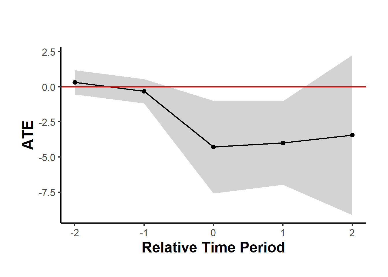
Figure 29.3: Event Study Plot of Average Treatment Effect Over Time (Subgroup)
Plot different estimators
library(causalverse)
methods <- c("synthdid", "did", "sc", "sc_ridge", "difp", "difp_ridge")

estimates <- lapply(methods, function(method) {
  synthdid_est_ate(
    data               = df,
    adoption_cohorts   = 5:7,
    lags               = 2,
    leads              = 2,
    time_var           = "year",
    unit_id_var        = "id",
    treated_period_var = "year_treated",
    treat_stat_var     = "treatvar",
    outcome_var        = "y",
    method = method
  )
})

plots <- lapply(seq_along(estimates), function(i) {
  causalverse::synthdid_plot_ate(estimates[[i]],
                                 title = methods[i],
                                 theme = causalverse::ama_theme(base_size = 6))
})

gridExtra::grid.arrange(grobs = plots, ncol = 2)