7 Generalized Linear Models
Generalized Linear Models (GLMs) extend the traditional linear regression framework to accommodate response variables that do not necessarily follow a normal distribution. They provide a flexible approach to modeling relationships between a set of predictors and various types of dependent variables.
While Ordinary Least Squares regression assumes that the response variable is continuous and normally distributed, GLMs allow for response variables that follow distributions from the exponential family, such as binomial, Poisson, and gamma distributions. This flexibility makes them particularly useful in a wide range of business and research applications.
A GLM consists of three key components:
- A random component: The response variable \(Y_i\) follows a distribution from the exponential family (e.g., binomial, Poisson, gamma).
- A systematic component: A linear predictor \(\eta_i = \mathbf{x'_i} \beta\), where \(\mathbf{x'_i}\) is a vector of observed covariates (predictor variables) and \(\beta\) is a vector of parameters to be estimated.
- A link function: A function \(g(\cdot)\) that relates the expected value of the response variable, \(\mu_i = E(Y_i)\), to the linear predictor (i.e., \(\eta_i = g(\mu_i)\)).
Although the relationship between the predictors and the outcome may appear nonlinear on the original outcome scale (due to the link function), a GLM is still considered “linear” in the statistical sense because it remains linear in the parameters \(\beta\). Consequently, GLMs are not generally classified as nonlinear regression models. They “generalize” the traditional linear model by allowing for a broader range of response variable distributions and link functions, but retain linearity in their parameters.
The choice of distribution and link function depends on the nature of the response variable. In the following sections, we will explore several important GLM variants:
- Logistic Regression: Used for binary response variables (e.g., customer churn, loan defaults).
- Probit Regression: Similar to logistic regression but assumes a normal distribution for the underlying probability.
- Poisson Regression: Used for modeling count data (e.g., number of purchases, call center inquiries).
- Negative Binomial Regression: An extension of Poisson regression that accounts for overdispersion in count data.
- Quasi-Poisson Regression: A variation of Poisson regression that adjusts for overdispersion by allowing the variance to be a linear function of the mean.
- Multinomial Logistic Regression: A generalization of logistic regression for categorical response variables with more than two outcomes.
- Generalization of Generalized Linear Model: A flexible generalization of ordinary linear regression that allows for response variables with different distributions (e.g., normal, binomial, Poisson).
7.1 Logistic Regression
Logistic regression is a widely used Generalized Linear Model designed for modeling binary response variables. It is particularly useful in applications such as credit scoring, medical diagnosis, and customer churn prediction.
7.1.1 Logistic Model
Given a set of predictor variables \(\mathbf{x}_i\), the probability of a positive outcome (e.g., success, event occurring) is modeled as:
\[ p_i = f(\mathbf{x}_i ; \beta) = \frac{\exp(\mathbf{x_i'\beta})}{1 + \exp(\mathbf{x_i'\beta})} \]
where:
- \(p_i = \mathbb{E}[Y_i]\) is the probability of success for observation \(i\).
- \(\mathbf{x_i}\) is the vector of predictor variables.
- \(\beta\) is the vector of model coefficients.
7.1.1.1 Logit Transformation
The logistic function can be rewritten in terms of the log-odds, also known as the logit function:
\[ \text{logit}(p_i) = \log \left(\frac{p_i}{1 - p_i} \right) = \mathbf{x_i'\beta} \]
where:
- \(\frac{p_i}{1 - p_i}\) represents the odds of success (the ratio of the probability of success to the probability of failure).
- The logit function ensures linearity in the parameters, which aligns with the GLM framework.
Thus, logistic regression belongs to the family of Generalized Linear Models because a function of the mean response (logit) is linear in the predictors.
7.1.2 Likelihood Function
Since \(Y_i\) follows a Bernoulli distribution with probability \(p_i\), the likelihood function for \(n\) independent observations is:
\[ L(p_i) = \prod_{i=1}^{n} p_i^{Y_i} (1 - p_i)^{1 - Y_i} \]
By substituting the logistic function for \(p_i\):
\[ p_i = \frac{\exp(\mathbf{x'_i \beta})}{1+\exp(\mathbf{x'_i \beta})}, \quad 1 - p_i = \frac{1}{1+\exp(\mathbf{x'_i \beta})} \]
we obtain:
\[ L(\beta) = \prod_{i=1}^{n} \left( \frac{\exp(\mathbf{x'_i \beta})}{1+\exp(\mathbf{x'_i \beta})} \right)^{Y_i} \left( \frac{1}{1+\exp(\mathbf{x'_i \beta})} \right)^{1 - Y_i} \]
Taking the natural logarithm of the likelihood function gives the log-likelihood function:
\[ Q(\beta) = \log L(\beta) = \sum_{i=1}^n Y_i \mathbf{x'_i \beta} - \sum_{i=1}^n \log(1 + \exp(\mathbf{x'_i \beta})) \]
Since this function is concave, we can maximize it numerically using iterative optimization techniques, such as:
- Newton-Raphson Algorithm
- Fisher Scoring Algorithm
These methods allow us to obtain the Maximum Likelihood Estimates of the parameters, \(\hat{\beta}\).
Under standard regularity conditions, the MLEs of logistic regression parameters are asymptotically normal:
\[ \hat{\beta} \dot{\sim} AN(\beta, [\mathbf{I}(\beta)]^{-1}) \]
where:
- \(\mathbf{I}(\beta)\) is the Fisher Information Matrix, which determines the variance-covariance structure of \(\hat{\beta}\).
7.1.3 Fisher Information Matrix
The Fisher Information Matrix quantifies the amount of information that an observable random variable carries about the unknown parameter \(\beta\). It is crucial in estimating the variance-covariance matrix of the estimated coefficients in logistic regression.
Mathematically, the Fisher Information Matrix is defined as:
\[ \mathbf{I}(\beta) = E\left[ \frac{\partial \log L(\beta)}{\partial \beta} \frac{\partial \log L(\beta)}{\partial \beta'} \right] \]
which expands to:
\[ \mathbf{I}(\beta) = E\left[ \left(\frac{\partial \log L(\beta)}{\partial \beta_i} \frac{\partial \log L(\beta)}{\partial \beta_j} \right)_{ij} \right] \]
Under regularity conditions, the Fisher Information Matrix is equivalent to the negative expected Hessian matrix:
\[ \mathbf{I}(\beta) = -E\left[ \frac{\partial^2 \log L(\beta)}{\partial \beta \partial \beta'} \right] \]
which further expands to:
\[ \mathbf{I}(\beta) = -E \left[ \left( \frac{\partial^2 \log L(\beta)}{\partial \beta_i \partial \beta_j} \right)_{ij} \right] \]
This representation is particularly useful because it allows us to compute the Fisher Information Matrix directly from the Hessian of the log-likelihood function.
Example: Fisher Information Matrix in Logistic Regression
Consider a simple logistic regression model with one predictor:
\[ x_i' \beta = \beta_0 + \beta_1 x_i \]
From the log-likelihood function, the second-order partial derivatives are:
\[ \begin{aligned} - \frac{\partial^2 \ln(L(\beta))}{\partial \beta^2_0} &= \sum_{i=1}^n \frac{\exp(x'_i \beta)}{1 + \exp(x'_i \beta)} - \left[\frac{\exp(x_i' \beta)}{1+ \exp(x'_i \beta)}\right]^2 & \text{Intercept} \\ &= \sum_{i=1}^n p_i (1-p_i) \\ - \frac{\partial^2 \ln(L(\beta))}{\partial \beta^2_1} &= \sum_{i=1}^n \frac{x_i^2\exp(x'_i \beta)}{1 + \exp(x'_i \beta)} - \left[\frac{x_i\exp(x_i' \beta)}{1+ \exp(x'_i \beta)}\right]^2 & \text{Slope}\\ &= \sum_{i=1}^n x_i^2p_i (1-p_i) \\ - \frac{\partial^2 \ln(L(\beta))}{\partial \beta_0 \partial \beta_1} &= \sum_{i=1}^n \frac{x_i\exp(x'_i \beta)}{1 + \exp(x'_i \beta)} - x_i\left[\frac{\exp(x_i' \beta)}{1+ \exp(x'_i \beta)}\right]^2 & \text{Cross-derivative}\\ &= \sum_{i=1}^n x_ip_i (1-p_i) \end{aligned} \]
Combining these elements, the Fisher Information Matrix for the logistic regression model is:
\[ \mathbf{I} (\beta) = \begin{bmatrix} \sum_{i=1}^{n} p_i(1 - p_i) & \sum_{i=1}^{n} x_i p_i(1 - p_i) \\ \sum_{i=1}^{n} x_i p_i(1 - p_i) & \sum_{i=1}^{n} x_i^2 p_i(1 - p_i) \end{bmatrix} \]
where:
- \(p_i = \frac{\exp(x_i' \beta)}{1+\exp(x_i' \beta)}\) represents the predicted probability.
- \(p_i (1 - p_i)\) is the variance of the Bernoulli response variable.
- The diagonal elements represent the variances of the estimated coefficients.
- The off-diagonal elements represent the covariances between \(\beta_0\) and \(\beta_1\).
The inverse of the Fisher Information Matrix provides the variance-covariance matrix of the estimated coefficients:
\[ \mathbf{Var}(\hat{\beta}) = \mathbf{I}(\hat{\beta})^{-1} \]
This matrix is essential for:
- Estimating standard errors of the logistic regression coefficients.
- Constructing confidence intervals for \(\beta\).
- Performing hypothesis tests (e.g., Wald Test).
# Load necessary library
library(stats)

# Simulated dataset
set.seed(123)
n <- 100
x <- rnorm(n)
y <- rbinom(n, 1, prob = plogis(0.5 + 1.2 * x))

# Fit logistic regression model
model <- glm(y ~ x, family = binomial)

# Extract the Fisher Information Matrix (Negative Hessian)
fisher_info <- summary(model)$cov.unscaled

# Display the Fisher Information Matrix
print(fisher_info)
#>             (Intercept)          x
#> (Intercept)  0.05718171 0.01564322
#> x            0.01564322 0.10302992
7.1.4 Inference in Logistic Regression
Once we estimate the model parameters \(\hat{\beta}\) using Maximum Likelihood Estimation, we can conduct inference to assess the significance of predictors, construct confidence intervals, and perform hypothesis testing. The two most common inference approaches in logistic regression are:
These tests rely on the asymptotic normality of MLEs and the properties of the Fisher Information Matrix.
7.1.4.1 Likelihood Ratio Test
The Likelihood Ratio Test compares two models:
- Restricted Model: A simpler model where some parameters are constrained to specific values.
- Unrestricted Model: The full model without constraints.
To test a hypothesis about a subset of parameters \(\beta_1\), we leave \(\beta_2\) (nuisance parameters) unspecified.
Hypothesis Setup:
\[ H_0: \beta_1 = \beta_{1,0} \]
where \(\beta_{1,0}\) is a specified value (often zero). Let:
- \(\hat{\beta}_{2,0}\) be the MLE of \(\beta_2\) under the constraint \(\beta_1 = \beta_{1,0}\).
- \(\hat{\beta}_1, \hat{\beta}_2\) be the MLEs under the full model.
The likelihood ratio test statistic is:
\[ -2\log\Lambda = -2[\log L(\beta_{1,0}, \hat{\beta}_{2,0}) - \log L(\hat{\beta}_1, \hat{\beta}_2)] \]
where:
- The first term is the log-likelihood of the restricted model.
- The second term is the log-likelihood of the unrestricted model.
Under the null hypothesis:
\[ -2 \log \Lambda \sim \chi^2_{\upsilon} \]
where \(\upsilon\) is the number of restricted parameters. We reject \(H_0\) if:
\[ -2\log \Lambda > \chi^2_{\upsilon,1-\alpha} \]
Interpretation: If the likelihood ratio test statistic is large, this suggests that the restricted model (under \(H_0\)) fits significantly worse than the full model, leading us to reject the null hypothesis.
7.1.4.2 Wald Test
The Wald test is based on the asymptotic normality of MLEs:
\[ \hat{\beta} \sim AN (\beta, [\mathbf{I}(\beta)]^{-1}) \]
We test:
\[ H_0: \mathbf{L} \hat{\beta} = 0 \]
where \(\mathbf{L}\) is a \(q \times p\) matrix with \(q\) linearly independent rows (often used to test multiple coefficients simultaneously). The Wald test statistic is:
\[ W = (\mathbf{L\hat{\beta}})'(\mathbf{L[I(\hat{\beta})]^{-1}L'})^{-1}(\mathbf{L\hat{\beta}}) \]
Under \(H_0\):
\[ W \sim \chi^2_q \]
Interpretation: If \(W\) is large, the null hypothesis is rejected, suggesting that at least one of the tested coefficients is significantly different from zero.
| Test | Best Used When… |
|---|---|
| Likelihood Ratio Test | More accurate in small samples, providing better control of error rates. Recommended when sample sizes are small. |
| Wald Test | Easier to compute but may be inaccurate in small samples. Recommended when computational efficiency is a priority. |
# Load necessary library
library(stats)

# Simulate some binary outcome data
set.seed(123)
n <- 100
x <- rnorm(n)
y <- rbinom(n, 1, prob = plogis(0.5 + 1.2 * x))

# Fit logistic regression model
model <- glm(y ~ x, family = binomial)

# Display model summary (includes Wald tests)
summary(model)
#>
#> Call:
#> glm(formula = y ~ x, family = binomial)
#>
#> Coefficients:
#>             Estimate Std. Error z value Pr(>|z|)
#> (Intercept)   0.7223     0.2391   3.020 0.002524 **
#> x             1.2271     0.3210   3.823 0.000132 ***
#> ---
#> Signif. codes:  0 '***' 0.001 '**' 0.01 '*' 0.05 '.' 0.1 ' ' 1
#>
#> (Dispersion parameter for binomial family taken to be 1)
#>
#>     Null deviance: 128.21  on 99  degrees of freedom
#> Residual deviance: 108.29  on 98  degrees of freedom
#> AIC: 112.29
#>
#> Number of Fisher Scoring iterations: 4

# Perform likelihood ratio test using anova()
anova(model, test="Chisq")
#> Analysis of Deviance Table
#>
#> Model: binomial, link: logit
#>
#> Response: y
#>
#> Terms added sequentially (first to last)
#>
#>
#>      Df Deviance Resid. Df Resid. Dev  Pr(>Chi)
#> NULL                    99     128.21
#> x     1   19.913        98     108.29 8.105e-06 ***
#> ---
#> Signif. codes:  0 '***' 0.001 '**' 0.01 '*' 0.05 '.' 0.1 ' ' 1
7.1.4.3 Confidence Intervals for Coefficients
A 95% confidence interval for a logistic regression coefficient \(\beta_i\) is given by:
\[ \hat{\beta}_i \pm 1.96 \hat{s}_{ii} \]
where:
- \(\hat{\beta}_i\) is the estimated coefficient.
- \(\hat{s}_{ii}\) is the standard error (square root of the diagonal element of \(\mathbf{[I(\hat{\beta})]}^{-1}\)).
This confidence interval provides a range of plausible values for \(\beta_i\). If the interval does not include zero, we conclude that \(\beta_i\) is statistically significant.
- For large sample sizes, the Likelihood Ratio Test and Wald Test yield similar results.
- For small sample sizes, the Likelihood Ratio Test is preferred because the Wald test can be less reliable.
7.1.4.4 Interpretation of Logistic Regression Coefficients
For a single predictor variable, the logistic regression model is:
\[ \text{logit}(\hat{p}_i) = \log\left(\frac{\hat{p}_i}{1 - \hat{p}_i} \right) = \hat{\beta}_0 + \hat{\beta}_1 x_i \]
where:
- \(\hat{p}_i\) is the predicted probability of success at \(x_i\).
- \(\hat{\beta}_1\) represents the log odds change for a one-unit increase in \(x\).
Interpreting \(\beta_1\) in Terms of Odds
When the predictor variable increases by one unit, the logit of the probability changes by \(\hat{\beta}_1\):
\[ \text{logit}(\hat{p}_{x_i +1}) = \hat{\beta}_0 + \hat{\beta}_1 (x_i + 1) = \text{logit}(\hat{p}_{x_i}) + \hat{\beta}_1 \]
Thus, the difference in log odds is:
\[ \begin{aligned} \text{logit}(\hat{p}_{x_i +1}) - \text{logit}(\hat{p}_{x_i}) &= \log ( \text{odds}(\hat{p}_{x_i + 1})) - \log (\text{odds}(\hat{p}_{x_i}) )\\ &= \log\left( \frac{\text{odds}(\hat{p}_{x_i + 1})}{\text{odds}(\hat{p}_{x_i})} \right) \\ &= \hat{\beta}_1 \end{aligned} \]
Exponentiating both sides:
\[ \exp(\hat{\beta}_1) = \frac{\text{odds}(\hat{p}_{x_i + 1})}{\text{odds}(\hat{p}_{x_i})} \]
This quantity, \(\exp(\hat{\beta}_1)\), is the odds ratio, which quantifies the effect of a one-unit increase in \(x\) on the odds of success.
Generalization: Odds Ratio for Any Change in \(x\)
For a difference of \(c\) units in the predictor \(x\), the estimated odds ratio is:
\[ \exp(c\hat{\beta}_1) \]
For multiple predictors, \(\exp(\hat{\beta}_k)\) represents the odds ratio for \(x_k\), holding all other variables constant.
7.1.4.5 Inference on the Mean Response
For a given set of predictor values \(x_h = (1, x_{h1}, ..., x_{h,p-1})'\), the estimated mean response (probability of success) is:
\[ \hat{p}_h = \frac{\exp(\mathbf{x'_h \hat{\beta}})}{1 + \exp(\mathbf{x'_h \hat{\beta}})} \]
The variance of the estimated probability is:
\[ s^2(\hat{p}_h) = \mathbf{x'_h[I(\hat{\beta})]^{-1}x_h} \]
where:
- \(\mathbf{I}(\hat{\beta})^{-1}\) is the variance-covariance matrix of \(\hat{\beta}\).
- \(s^2(\hat{p}_h)\) provides an estimate of uncertainty in \(\hat{p}_h\).
In many applications, logistic regression is used for classification, where we predict whether an observation belongs to category 0 or 1. A commonly used decision rule is:
- Assign \(y = 1\) if \(\hat{p}_h \geq \tau\)
- Assign \(y = 0\) if \(\hat{p}_h < \tau\)
where \(\tau\) is a chosen cutoff threshold (typically \(\tau = 0.5\)).
# Load necessary library
library(stats)

# Simulated dataset
set.seed(123)
n <- 100
x <- rnorm(n)
y <- rbinom(n, 1, prob = plogis(0.5 + 1.2 * x))

# Fit logistic regression model
model <- glm(y ~ x, family = binomial)

# Display model summary
summary(model)
#>
#> Call:
#> glm(formula = y ~ x, family = binomial)
#>
#> Coefficients:
#>             Estimate Std. Error z value Pr(>|z|)
#> (Intercept)   0.7223     0.2391   3.020 0.002524 **
#> x             1.2271     0.3210   3.823 0.000132 ***
#> ---
#> Signif. codes:  0 '***' 0.001 '**' 0.01 '*' 0.05 '.' 0.1 ' ' 1
#>
#> (Dispersion parameter for binomial family taken to be 1)
#>
#>     Null deviance: 128.21  on 99  degrees of freedom
#> Residual deviance: 108.29  on 98  degrees of freedom
#> AIC: 112.29
#>
#> Number of Fisher Scoring iterations: 4

# Extract coefficients and standard errors
coef_estimates <- coef(summary(model))
beta_hat <- coef_estimates[, 1]   # Estimated coefficients
se_beta  <- coef_estimates[, 2]   # Standard errors

# Compute 95% confidence intervals for coefficients
conf_intervals <- cbind(
  beta_hat - 1.96 * se_beta,
  beta_hat + 1.96 * se_beta
)

# Compute Odds Ratios
odds_ratios <- exp(beta_hat)

# Display results
print("Confidence Intervals for Coefficients:")
#> [1] "Confidence Intervals for Coefficients:"
print(conf_intervals)
#>                  [,1]     [,2]
#> (Intercept) 0.2535704 1.190948
#> x           0.5979658 1.856218

print("Odds Ratios:")
#> [1] "Odds Ratios:"
print(odds_ratios)
#> (Intercept)           x
#>    2.059080    3.411295

# Predict probability for a new observation (e.g., x = 1)
new_x <- data.frame(x = 1)
predicted_prob <- predict(model, newdata = new_x, type = "response")

print("Predicted Probability for x = 1:")
#> [1] "Predicted Probability for x = 1:"
print(predicted_prob)
#>         1
#> 0.8753759
7.1.5 Application: Logistic Regression
In this section, we demonstrate the application of logistic regression using simulated data. We explore model fitting, inference, residual analysis, and goodness-of-fit testing.
1. Load Required Libraries
library(kableExtra)
library(dplyr)
library(pscl)
library(ggplot2)
library(faraway)
library(nnet)
library(agridat)
library(nlstools)
2. Data Generation
We generate a dataset where the predictor variable \(X\) follows a uniform distribution:
\[ x \sim Unif(-0.5,2.5) \]
The linear predictor is given by:
\[ \eta = 0.5 + 0.75 x \]
Passing \(\eta\) into the inverse-logit function, we obtain:
\[ p = \frac{\exp(\eta)}{1+ \exp(\eta)} \]
which ensures that \(p \in [0,1]\). We then generate the binary response variable:
\[ y \sim Bernoulli(p) \]
set.seed(23) # Set seed for reproducibility
x <- runif(1000, min = -0.5, max = 2.5)  # Generate X values
eta1 <- 0.5 + 0.75 * x                   # Compute linear predictor
p <- exp(eta1) / (1 + exp(eta1))          # Compute probabilities
y <- rbinom(1000, 1, p)                   # Generate binary response
BinData <- data.frame(X = x, Y = y)       # Create data frame
3. Model Fitting
We fit a logistic regression model to the simulated data:
\[ \text{logit}(p) = \beta_0 + \beta_1 X \]
Logistic_Model <- glm(formula = Y ~ X,
                      # Specifies the response distribution
                      family = binomial,
                      data = BinData)

summary(Logistic_Model) # Model summary
#>
#> Call:
#> glm(formula = Y ~ X, family = binomial, data = BinData)
#>
#> Coefficients:
#>             Estimate Std. Error z value Pr(>|z|)
#> (Intercept)  0.46205    0.10201   4.530 5.91e-06 ***
#> X            0.78527    0.09296   8.447  < 2e-16 ***
#> ---
#> Signif. codes:  0 '***' 0.001 '**' 0.01 '*' 0.05 '.' 0.1 ' ' 1
#>
#> (Dispersion parameter for binomial family taken to be 1)
#>
#>     Null deviance: 1106.7  on 999  degrees of freedom
#> Residual deviance: 1027.4  on 998  degrees of freedom
#> AIC: 1031.4
#>
#> Number of Fisher Scoring iterations: 4
nlstools::confint2(Logistic_Model) # Confidence intervals
#>                 2.5 %    97.5 %
#> (Intercept) 0.2618709 0.6622204
#> X           0.6028433 0.9676934

# Compute odds ratios
OddsRatio <- coef(Logistic_Model) %>% exp
OddsRatio
#> (Intercept)           X
#>    1.587318    2.192995
Interpretation of the Odds Ratio
When \(x = 0\), the odds of success are 1.59.
When \(x = 1\), the odds of success increase by a factor of 2.19, indicating a 119.29% increase.
4. Deviance Test
We assess the model’s significance using the deviance test, which compares:
\(H_0\): No predictors are related to the response (intercept-only model).
\(H_1\): At least one predictor is related to the response.
The test statistic is:
\[ D = \text{Null Deviance} - \text{Residual Deviance} \]
Test_Dev <- Logistic_Model$null.deviance - Logistic_Model$deviance
p_val_dev <- 1 - pchisq(q = Test_Dev, df = 1)
p_val_dev
#> [1] 0
Since the p-value is approximately 0, we reject \(H_0\), confirming that \(X\) is significantly related to \(Y\).
5. Residual Analysis
We compute deviance residuals and plot them against \(X\).
Logistic_Resids <- residuals(Logistic_Model, type = "deviance")
plot(
    y = Logistic_Resids,
    x = BinData$X,
    xlab = 'X',
    ylab = 'Deviance Residuals'
)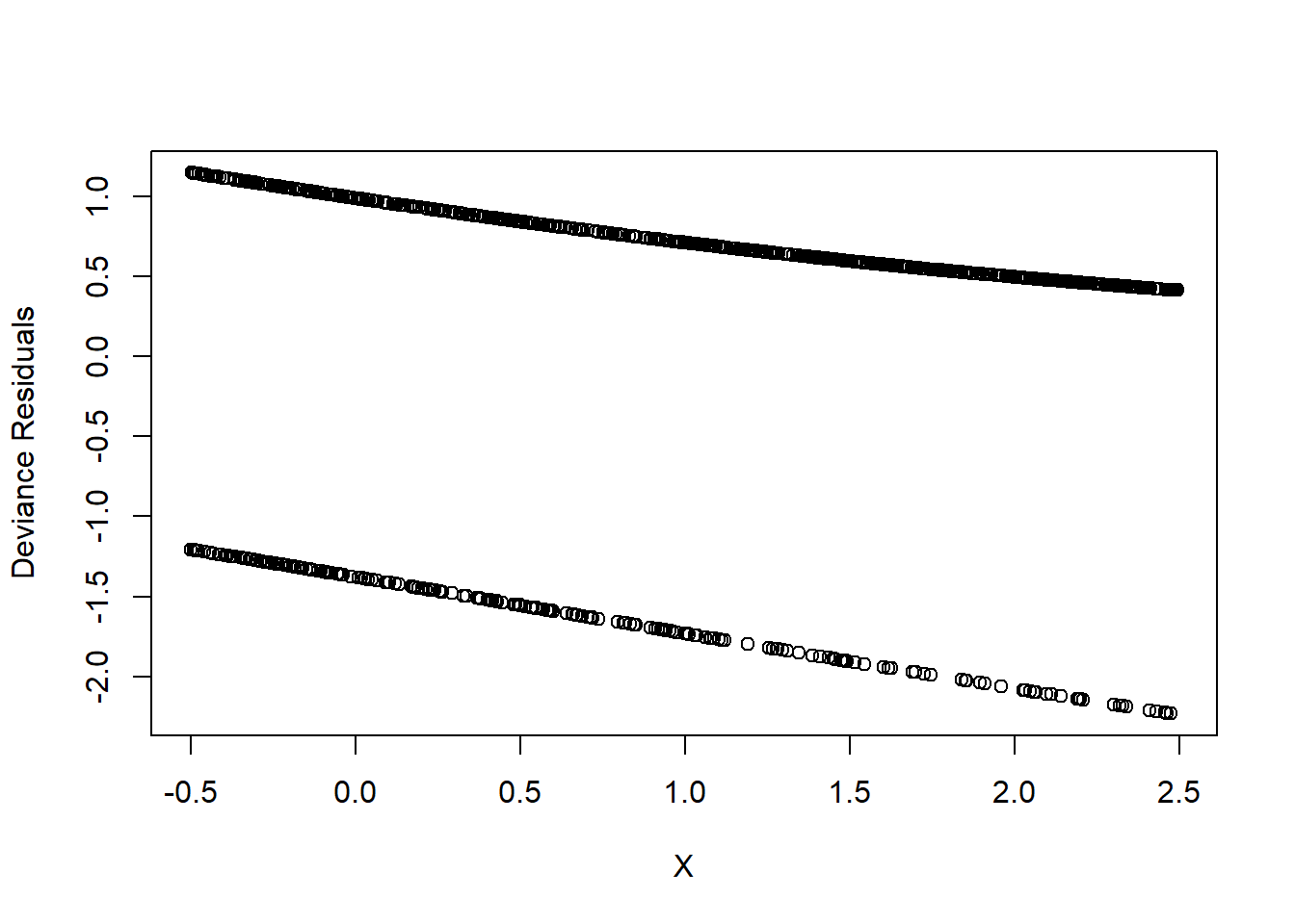
Figure 7.1: Deviance Residuals
This plot is not very informative. A more insightful approach is binned residual plots.
6. Binned Residual Plot
We group residuals into bins based on predicted values.
plot_bin <- function(Y,
                     X,
                     bins = 100,
                     return.DF = FALSE) {
  Y_Name <- deparse(substitute(Y))
  X_Name <- deparse(substitute(X))

  Binned_Plot <- data.frame(Plot_Y = Y, Plot_X = X)
  Binned_Plot$bin <-
    cut(Binned_Plot$Plot_X, breaks = bins) %>% as.numeric

  Binned_Plot_summary <- Binned_Plot %>%
    group_by(bin) %>%
    summarise(
      Y_ave = mean(Plot_Y),
      X_ave = mean(Plot_X),
      Count = n()
    ) %>% as.data.frame

  plot(
    y = Binned_Plot_summary$Y_ave,
    x = Binned_Plot_summary$X_ave,
    ylab = Y_Name,
    xlab = X_Name
  )

  if (return.DF)
    return(Binned_Plot_summary)
}

plot_bin(Y = Logistic_Resids, X = BinData$X, bins = 100)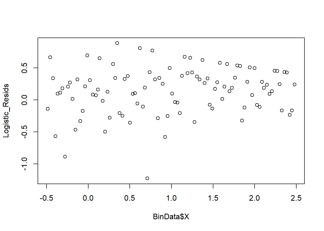
Figure 7.2: Binned Residual Plot
We also examine predicted values vs residuals:
Logistic_Predictions <- predict(Logistic_Model, type = "response")
plot_bin(Y = Logistic_Resids, X = Logistic_Predictions, bins = 100)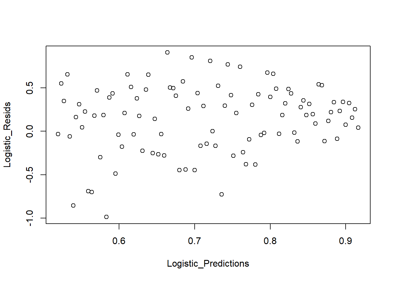
Figure 7.3: Predicted Values versus Residuals
Finally, we compare predicted probabilities to actual outcomes:
NumBins <- 10
Binned_Data <- plot_bin(
    Y = BinData$Y,
    X = Logistic_Predictions,
    bins = NumBins,
    return.DF = TRUE
)
Binned_Data
#>    bin     Y_ave     X_ave Count
#> 1    1 0.5833333 0.5382095    72
#> 2    2 0.5200000 0.5795887    75
#> 3    3 0.6567164 0.6156540    67
#> 4    4 0.7014925 0.6579674    67
#> 5    5 0.6373626 0.6984765    91
#> 6    6 0.7500000 0.7373341    72
#> 7    7 0.7096774 0.7786747    93
#> 8    8 0.8503937 0.8203819   127
#> 9    9 0.8947368 0.8601232   133
#> 10  10 0.8916256 0.9004734   203
abline(0, 1, lty = 2, col = 'blue')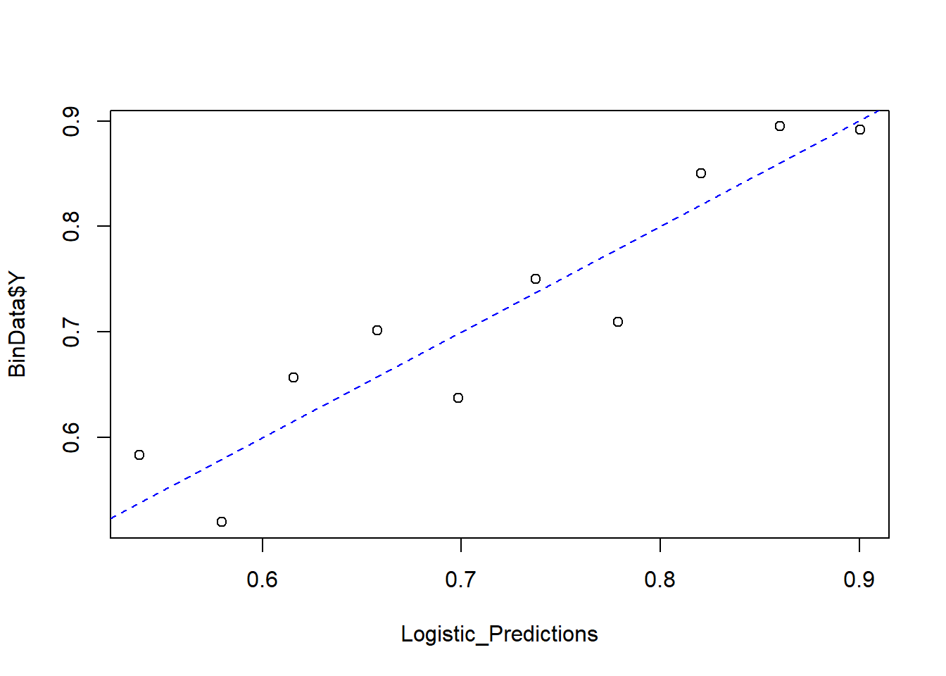
Figure 7.4: Predicted versus Actual Values
7. Model Goodness-of-Fit: Hosmer-Lemeshow Test
The Hosmer-Lemeshow test evaluates whether the model fits the data well. The test statistic is: \[ X^2_{HL} = \sum_{j=1}^{J} \frac{(y_j - m_j \hat{p}_j)^2}{m_j \hat{p}_j(1-\hat{p}_j)} \] where:
\(y_j\) is the observed number of successes in bin \(j\).
\(m_j\) is the number of observations in bin \(j\).
\(\hat{p}_j\) is the predicted probability in bin \(j\).
Under \(H_0\), we assume:
\[ X^2_{HL} \sim \chi^2_{J-1} \]
HL_BinVals <- (Binned_Data$Count * Binned_Data$Y_ave -
               Binned_Data$Count * Binned_Data$X_ave) ^ 2 /
               (Binned_Data$Count * Binned_Data$X_ave * (1 - Binned_Data$X_ave))

HLpval <- pchisq(q = sum(HL_BinVals),
                 df = NumBins - 1,
                 lower.tail = FALSE)
HLpval
#> [1] 0.4150004
Conclusion:
Since \(p\)-value = 0.99, we fail to reject \(H_0\).
This indicates that the model fits the data well.
7.2 Probit Regression
Probit regression is a type of Generalized Linear Models used for binary outcome variables. Unlike logistic regression, which uses the logit function, probit regression assumes that the probability of success is determined by an underlying normally distributed latent variable.
7.2.1 Probit Model
Let \(Y_i\) be a binary response variable:
\[ Y_i = \begin{cases} 1, & \text{if success occurs} \\ 0, & \text{otherwise} \end{cases} \]
We assume that \(Y_i\) follows a Bernoulli distribution:
\[ Y_i \sim \text{Bernoulli}(p_i), \quad \text{where } p_i = P(Y_i = 1 | \mathbf{x_i}) \]
Instead of the logit function in logistic regression:
\[ \text{logit}(p_i) = \log\left( \frac{p_i}{1 - p_i} \right) = \mathbf{x_i'\beta} \]
Probit regression uses the inverse standard normal CDF:
\[ \Phi^{-1}(p_i) = \mathbf{x_i'\theta} \]
where:
\(\Phi(\cdot)\) is the CDF of the standard normal distribution.
\(\mathbf{x_i}\) is the vector of predictors.
\(\theta\) is the vector of regression coefficients.
Thus, the probability of success is:
\[ p_i = P(Y_i = 1 | \mathbf{x_i}) = \Phi(\mathbf{x_i'\theta}) \]
where:
\[ \Phi(z) = \int_{-\infty}^{z} \frac{1}{\sqrt{2\pi}} e^{-t^2/2} dt \]
7.2.2 Application: Probit Regression
# Load necessary library
library(ggplot2)

# Set seed for reproducibility
set.seed(123)

# Simulate data
n <- 1000
x1 <- rnorm(n)
x2 <- rnorm(n)
latent <- 0.5 * x1 + 0.7 * x2 + rnorm(n)  # Linear combination
y <- ifelse(latent > 0, 1, 0)  # Binary outcome

# Create dataframe
data <- data.frame(y, x1, x2)

# Fit Probit model
probit_model <-
    glm(y ~ x1 + x2, family = binomial(link = "probit"), data = data)
summary(probit_model)
#>
#> Call:
#> glm(formula = y ~ x1 + x2, family = binomial(link = "probit"),
#>     data = data)
#>
#> Coefficients:
#>             Estimate Std. Error z value Pr(>|z|)
#> (Intercept) -0.09781    0.04499  -2.174   0.0297 *
#> x1           0.43838    0.04891   8.963   <2e-16 ***
#> x2           0.75538    0.05306  14.235   <2e-16 ***
#> ---
#> Signif. codes:  0 '***' 0.001 '**' 0.01 '*' 0.05 '.' 0.1 ' ' 1
#>
#> (Dispersion parameter for binomial family taken to be 1)
#>
#>     Null deviance: 1385.1  on 999  degrees of freedom
#> Residual deviance: 1045.3  on 997  degrees of freedom
#> AIC: 1051.3
#>
#> Number of Fisher Scoring iterations: 5

# Fit Logit model
logit_model <-
    glm(y ~ x1 + x2, family = binomial(link = "logit"), data = data)
summary(logit_model)
#>
#> Call:
#> glm(formula = y ~ x1 + x2, family = binomial(link = "logit"),
#>     data = data)
#>
#> Coefficients:
#>             Estimate Std. Error z value Pr(>|z|)
#> (Intercept) -0.16562    0.07600  -2.179   0.0293 *
#> x1           0.73234    0.08507   8.608   <2e-16 ***
#> x2           1.25220    0.09486  13.201   <2e-16 ***
#> ---
#> Signif. codes:  0 '***' 0.001 '**' 0.01 '*' 0.05 '.' 0.1 ' ' 1
#>
#> (Dispersion parameter for binomial family taken to be 1)
#>
#>     Null deviance: 1385.1  on 999  degrees of freedom
#> Residual deviance: 1048.4  on 997  degrees of freedom
#> AIC: 1054.4
#>
#> Number of Fisher Scoring iterations: 4

# Compare Coefficients
coef_comparison <- data.frame(
    Variable = names(coef(probit_model)),
    Probit_Coef = coef(probit_model),
    Logit_Coef = coef(logit_model),
    Logit_Probit_Ratio = coef(logit_model) / coef(probit_model)
)

print(coef_comparison)
#>                Variable Probit_Coef Logit_Coef Logit_Probit_Ratio
#> (Intercept) (Intercept) -0.09780689 -0.1656216           1.693353
#> x1                   x1  0.43837627  0.7323392           1.670572
#> x2                   x2  0.75538259  1.2522008           1.657704

# Compute predicted probabilities
data$probit_pred <- predict(probit_model, type = "response")
data$logit_pred <- predict(logit_model, type = "response")
# Plot Probit vs Logit predictions
ggplot(data, aes(x = probit_pred, y = logit_pred)) +
  geom_point(alpha = 0.5) +
  geom_abline(slope = 1,
              intercept = 0,
              col = "red") +
  labs(title = "Comparison of Predicted Probabilities",
       x = "Probit Predictions", y = "Logit Predictions")
Figure 7.5: Comparison of Predicted Probabilities
# Classification Accuracy
threshold <- 0.5
data$probit_class <- ifelse(data$probit_pred > threshold, 1, 0)
data$logit_class <- ifelse(data$logit_pred > threshold, 1, 0)

probit_acc <- mean(data$probit_class == data$y)
logit_acc <- mean(data$logit_class == data$y)

print(paste("Probit Accuracy:", round(probit_acc, 4)))
#> [1] "Probit Accuracy: 0.71"
print(paste("Logit Accuracy:", round(logit_acc, 4)))
#> [1] "Logit Accuracy: 0.71"
7.3 Binomial Regression
In previous sections, we introduced binomial regression models, including both Logistic Regression and probit regression, and discussed their theoretical foundations. Now, we apply these methods to real-world data using the esoph dataset, which examines the relationship between esophageal cancer and potential risk factors such as alcohol consumption and age group.
7.3.1 Dataset Overview
The esoph dataset consists of:
Successes (
ncases): The number of individuals diagnosed with esophageal cancer.Failures (
ncontrols): The number of individuals in the control group (without cancer).-
Predictors:
agegp: Age group of individuals.alcgp: Alcohol consumption category.tobgp: Tobacco consumption category.
Before fitting our models, let’s inspect the dataset and visualize some key relationships.
# Load and inspect the dataset
data("esoph")
head(esoph, n = 3)
#>   agegp     alcgp    tobgp ncases ncontrols
#> 1 25-34 0-39g/day 0-9g/day      0        40
#> 2 25-34 0-39g/day    10-19      0        10
#> 3 25-34 0-39g/day    20-29      0         6
# Visualizing the proportion of cancer cases by alcohol consumption
plot(
  esoph$ncases / (esoph$ncases + esoph$ncontrols) ~ esoph$alcgp,
  ylab = "Proportion of Cancer Cases",
  xlab = "Alcohol Consumption Group",
  main = "Esophageal Cancer Data"
)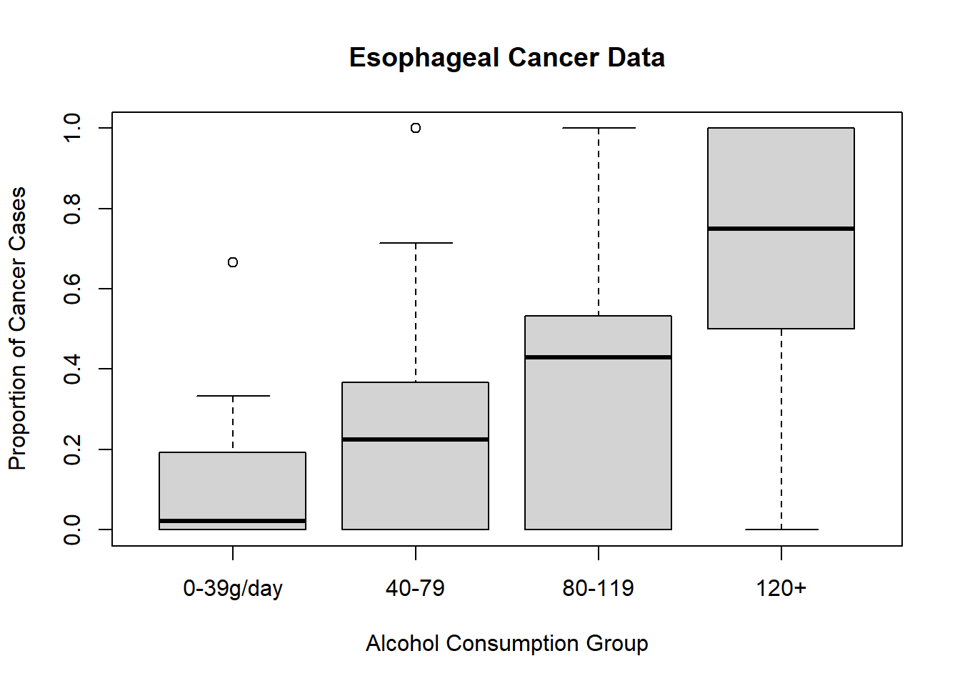
Figure 7.6: Esophageal Cancer Data
7.3.2 Apply Logistic Model
We first fit a logistic regression model, where the response variable is the proportion of cancer cases (ncases) relative to total observations (ncases + ncontrols).
# Logistic regression using alcohol consumption as a predictor
model <-
    glm(cbind(ncases, ncontrols) ~ alcgp,
        data = esoph,
        family = binomial)

# Summary of the model
summary(model)
#>
#> Call:
#> glm(formula = cbind(ncases, ncontrols) ~ alcgp, family = binomial,
#>     data = esoph)
#>
#> Coefficients:
#>             Estimate Std. Error z value Pr(>|z|)
#> (Intercept)  -2.5885     0.1925 -13.444  < 2e-16 ***
#> alcgp40-79    1.2712     0.2323   5.472 4.46e-08 ***
#> alcgp80-119   2.0545     0.2611   7.868 3.59e-15 ***
#> alcgp120+     3.3042     0.3237  10.209  < 2e-16 ***
#> ---
#> Signif. codes:  0 '***' 0.001 '**' 0.01 '*' 0.05 '.' 0.1 ' ' 1
#>
#> (Dispersion parameter for binomial family taken to be 1)
#>
#>     Null deviance: 367.95  on 87  degrees of freedom
#> Residual deviance: 221.46  on 84  degrees of freedom
#> AIC: 344.51
#>
#> Number of Fisher Scoring iterations: 5
Interpretation
The coefficients represent the log-odds of having esophageal cancer relative to the baseline alcohol consumption group.
P-values indicate whether alcohol consumption levels significantly influence cancer risk.
Model Diagnostics
# Convert coefficients to odds ratios
exp(coefficients(model))
#> (Intercept)  alcgp40-79 alcgp80-119   alcgp120+
#>  0.07512953  3.56527094  7.80261593 27.22570533

# Model goodness-of-fit measures
deviance(model) / df.residual(model)  # Closer to 1 suggests a better fit
#> [1] 2.63638
model$aic  # Lower AIC is preferable for model comparison
#> [1] 344.5109
To improve our model, we include age group (agegp) as an additional predictor.
# Logistic regression with alcohol consumption and age
better_model <- glm(
    cbind(ncases, ncontrols) ~ agegp + alcgp,
    data = esoph,
    family = binomial
)

# Summary of the improved model
summary(better_model)
#>
#> Call:
#> glm(formula = cbind(ncases, ncontrols) ~ agegp + alcgp, family = binomial,
#>     data = esoph)
#>
#> Coefficients:
#>             Estimate Std. Error z value Pr(>|z|)
#> (Intercept)  -6.1472     1.0419  -5.900 3.63e-09 ***
#> agegp35-44    1.6311     1.0800   1.510 0.130973
#> agegp45-54    3.4258     1.0389   3.297 0.000976 ***
#> agegp55-64    3.9435     1.0346   3.811 0.000138 ***
#> agegp65-74    4.3568     1.0413   4.184 2.87e-05 ***
#> agegp75+      4.4242     1.0914   4.054 5.04e-05 ***
#> alcgp40-79    1.4343     0.2448   5.859 4.64e-09 ***
#> alcgp80-119   2.0071     0.2776   7.230 4.84e-13 ***
#> alcgp120+     3.6800     0.3763   9.778  < 2e-16 ***
#> ---
#> Signif. codes:  0 '***' 0.001 '**' 0.01 '*' 0.05 '.' 0.1 ' ' 1
#>
#> (Dispersion parameter for binomial family taken to be 1)
#>
#>     Null deviance: 367.95  on 87  degrees of freedom
#> Residual deviance: 105.88  on 79  degrees of freedom
#> AIC: 238.94
#>
#> Number of Fisher Scoring iterations: 6

# Model evaluation
better_model$aic # Lower AIC is better
#> [1] 238.9361

# Convert coefficients to odds ratios
# exp(coefficients(better_model))
data.frame(`Odds Ratios` = exp(coefficients(better_model)))
#>              Odds.Ratios
#> (Intercept)  0.002139482
#> agegp35-44   5.109601844
#> agegp45-54  30.748594216
#> agegp55-64  51.596634690
#> agegp65-74  78.005283850
#> agegp75+    83.448437749
#> alcgp40-79   4.196747169
#> alcgp80-119  7.441782227
#> alcgp120+   39.646885126

# Compare models using likelihood ratio test (Chi-square test)
pchisq(
    q = model$deviance - better_model$deviance,
    df = model$df.residual - better_model$df.residual,
    lower.tail = FALSE
)
#> [1] 2.713923e-23
Key Takeaways
AIC Reduction: A lower AIC suggests that adding age as a predictor improves the model.
Likelihood Ratio Test: This test compares the two models and determines whether the improvement is statistically significant.
7.3.3 Apply Probit Model
As discussed earlier, the probit model is an alternative to logistic regression, using a cumulative normal distribution instead of the logistic function.
# Probit regression model
Prob_better_model <- glm(
    cbind(ncases, ncontrols) ~ agegp + alcgp,
    data = esoph,
    family = binomial(link = probit)
)

# Summary of the probit model
summary(Prob_better_model)
#>
#> Call:
#> glm(formula = cbind(ncases, ncontrols) ~ agegp + alcgp, family = binomial(link = probit),
#>     data = esoph)
#>
#> Coefficients:
#>             Estimate Std. Error z value Pr(>|z|)
#> (Intercept)  -3.3741     0.4922  -6.855 7.13e-12 ***
#> agegp35-44    0.8562     0.5081   1.685 0.092003 .
#> agegp45-54    1.7829     0.4904   3.636 0.000277 ***
#> agegp55-64    2.1034     0.4876   4.314 1.61e-05 ***
#> agegp65-74    2.3374     0.4930   4.741 2.13e-06 ***
#> agegp75+      2.3694     0.5275   4.491 7.08e-06 ***
#> alcgp40-79    0.8080     0.1330   6.076 1.23e-09 ***
#> alcgp80-119   1.1399     0.1558   7.318 2.52e-13 ***
#> alcgp120+     2.1204     0.2060  10.295  < 2e-16 ***
#> ---
#> Signif. codes:  0 '***' 0.001 '**' 0.01 '*' 0.05 '.' 0.1 ' ' 1
#>
#> (Dispersion parameter for binomial family taken to be 1)
#>
#>     Null deviance: 367.95  on 87  degrees of freedom
#> Residual deviance: 104.48  on 79  degrees of freedom
#> AIC: 237.53
#>
#> Number of Fisher Scoring iterations: 6
Why Consider a Probit Model?
Like logistic regression, probit regression estimates probabilities, but it assumes a normal distribution of the latent variable.
While the interpretation of coefficients differs, model comparisons can still be made using AIC.
7.4 Poisson Regression
7.4.1 The Poisson Distribution
Poisson regression is used for modeling count data, where the response variable represents the number of occurrences of an event within a fixed period, space, or other unit. The Poisson distribution is defined as:
\[ \begin{aligned} f(Y_i) &= \frac{\mu_i^{Y_i} \exp(-\mu_i)}{Y_i!}, \quad Y_i = 0,1,2, \dots \\ E(Y_i) &= \mu_i \\ \text{Var}(Y_i) &= \mu_i \end{aligned} \] where:
\(Y_i\) is the count variable.
\(\mu_i\) is the expected count for the \(i\)-th observation.
The mean and variance are equal \(E(Y_i) = \text{Var}(Y_i)\), making Poisson regression suitable when variance follows this property.
However, real-world count data often exhibit overdispersion, where the variance exceeds the mean. We will discuss remedies such as Quasi-Poisson and Negative Binomial Regression later.
7.4.2 Poisson Model
We model the expected count \(\mu_i\) as a function of predictors \(\mathbf{x_i}\) and parameters \(\boldsymbol{\theta}\):
\[ \mu_i = f(\mathbf{x_i; \theta}) \]
7.4.3 Link Function Choices
Since \(\mu_i\) must be positive, we often use a log-link function:
\[ θ\log(\mu_i) = \mathbf{x_i' \theta} \]
This ensures that the predicted counts are always non-negative. This is analogous to logistic regression, where we use the logit link for binary outcomes.
Rewriting:
\[ \mu_i = \exp(\mathbf{x_i' \theta}) \] which ensures \(\mu_i > 0\) for all parameter values.
7.4.4 Application: Poisson Regression
We apply Poisson regression to the bioChemists dataset (from the pscl package), which contains information on academic productivity in terms of published articles.
7.4.4.1 Dataset Overview
library(tidyverse)
# Load dataset
data(bioChemists, package = "pscl")

# Rename columns for clarity
bioChemists <- bioChemists %>%
  rename(
    Num_Article = art,
    # Number of articles in last 3 years
    Sex = fem,
    # 1 if female, 0 if male
    Married = mar,
    # 1 if married, 0 otherwise
    Num_Kid5 = kid5,
    # Number of children under age 6
    PhD_Quality = phd,
    # Prestige of PhD program
    Num_MentArticle = ment   # Number of articles by mentor in last 3 years
  )
# Visualize response variable distribution
hist(bioChemists$Num_Article,
     breaks = 25,
     main = "Number of Articles Published")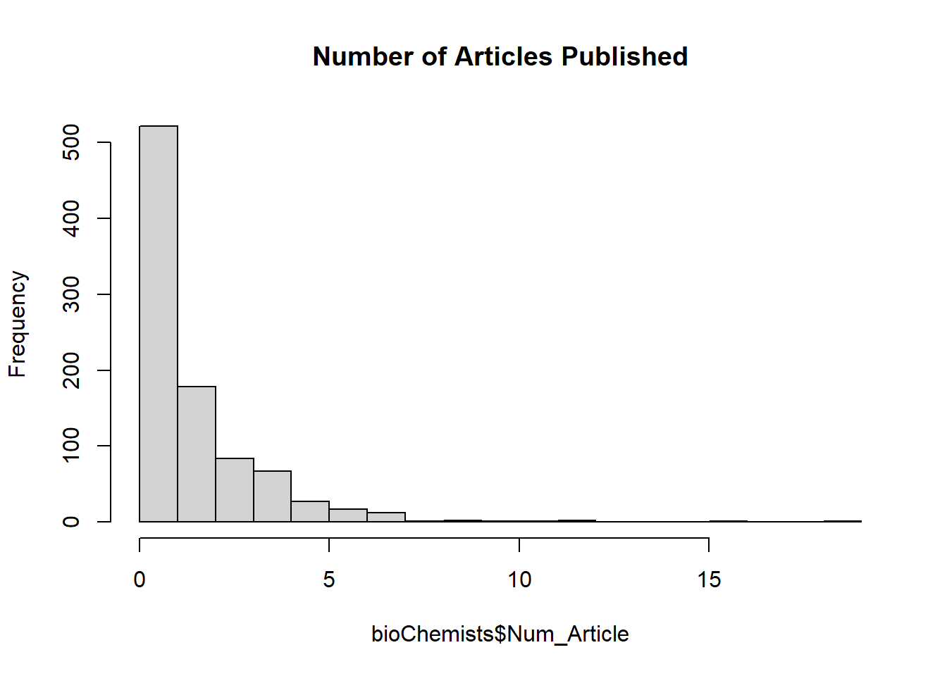
Figure 7.7: Number of Articles Published
The distribution of the number of articles is right-skewed, which suggests a Poisson model may be appropriate.
7.4.4.2 Fitting a Poisson Regression Model
We model the number of articles published (Num_Article) as a function of various predictors.
# Poisson regression model
Poisson_Mod <-
  glm(Num_Article ~ .,
      family = poisson,
      data = bioChemists)

# Summary of the model
summary(Poisson_Mod)
#>
#> Call:
#> glm(formula = Num_Article ~ ., family = poisson, data = bioChemists)
#>
#> Coefficients:
#>                  Estimate Std. Error z value Pr(>|z|)
#> (Intercept)      0.304617   0.102981   2.958   0.0031 **
#> SexWomen        -0.224594   0.054613  -4.112 3.92e-05 ***
#> MarriedMarried   0.155243   0.061374   2.529   0.0114 *
#> Num_Kid5        -0.184883   0.040127  -4.607 4.08e-06 ***
#> PhD_Quality      0.012823   0.026397   0.486   0.6271
#> Num_MentArticle  0.025543   0.002006  12.733  < 2e-16 ***
#> ---
#> Signif. codes:  0 '***' 0.001 '**' 0.01 '*' 0.05 '.' 0.1 ' ' 1
#>
#> (Dispersion parameter for poisson family taken to be 1)
#>
#>     Null deviance: 1817.4  on 914  degrees of freedom
#> Residual deviance: 1634.4  on 909  degrees of freedom
#> AIC: 3314.1
#>
#> Number of Fisher Scoring iterations: 5
Interpretation:
Coefficients are on the log scale, meaning they represent log-rate ratios.
Exponentiating the coefficients gives the rate ratios.
Statistical significance tells us whether each variable has a meaningful impact on publication count.
7.4.4.3 Model Diagnostics: Goodness of Fit
7.4.4.3.1 Pearson’s Chi-Square Test for Overdispersion
We compute the Pearson chi-square statistic to check whether the variance significantly exceeds the mean.
\[ X^2 = \sum \frac{(Y_i - \hat{\mu}_i)^2}{\hat{\mu}_i} \]
# Compute predicted means
Predicted_Means <- predict(Poisson_Mod, type = "response")

# Pearson chi-square test
X2 <-
  sum((bioChemists$Num_Article - Predicted_Means) ^ 2 / Predicted_Means)
X2
#> [1] 1662.547
pchisq(X2, Poisson_Mod$df.residual, lower.tail = FALSE)
#> [1] 7.849882e-47
If p-value is small, overdispersion is present.
Large X² statistic suggests the model may not adequately capture variability.
7.4.4.3.2 Overdispersion Check: Ratio of Deviance to Degrees of Freedom
We compute:
\[ \hat{\phi} = \frac{\text{deviance}}{\text{degrees of freedom}} \]
# Overdispersion check
Poisson_Mod$deviance / Poisson_Mod$df.residual
#> [1] 1.797988
If \(\hat{\phi} > 1\), overdispersion is likely present.
A value significantly above 1 suggests the need for an alternative model.
7.4.4.4 Addressing Overdispersion
7.4.4.4.1 Including Interaction Terms
One possible remedy is to incorporate interaction terms, capturing complex relationships between predictors.
# Adding two-way and three-way interaction terms
Poisson_Mod_All2way <-
  glm(Num_Article ~ . ^ 2, family = poisson, data = bioChemists)
Poisson_Mod_All3way <-
  glm(Num_Article ~ . ^ 3, family = poisson, data = bioChemists)
This may improve model fit, but can lead to overfitting.
7.4.4.4.2 Quasi-Poisson Model (Adjusting for Overdispersion)
A quick fix is to allow the variance to scale by introducing \(\hat{\phi}\):
\[ \text{Var}(Y_i) = \hat{\phi} \mu_i \]
# Estimate dispersion parameter
phi_hat = Poisson_Mod$deviance / Poisson_Mod$df.residual

# Adjusting Poisson model to account for overdispersion
summary(Poisson_Mod, dispersion = phi_hat)
#>
#> Call:
#> glm(formula = Num_Article ~ ., family = poisson, data = bioChemists)
#>
#> Coefficients:
#>                 Estimate Std. Error z value Pr(>|z|)
#> (Intercept)      0.30462    0.13809   2.206  0.02739 *
#> SexWomen        -0.22459    0.07323  -3.067  0.00216 **
#> MarriedMarried   0.15524    0.08230   1.886  0.05924 .
#> Num_Kid5        -0.18488    0.05381  -3.436  0.00059 ***
#> PhD_Quality      0.01282    0.03540   0.362  0.71715
#> Num_MentArticle  0.02554    0.00269   9.496  < 2e-16 ***
#> ---
#> Signif. codes:  0 '***' 0.001 '**' 0.01 '*' 0.05 '.' 0.1 ' ' 1
#>
#> (Dispersion parameter for poisson family taken to be 1.797988)
#>
#>     Null deviance: 1817.4  on 914  degrees of freedom
#> Residual deviance: 1634.4  on 909  degrees of freedom
#> AIC: 3314.1
#>
#> Number of Fisher Scoring iterations: 5
Alternatively, we refit using a Quasi-Poisson model, which adjusts standard errors:
# Quasi-Poisson model
quasiPoisson_Mod <- glm(Num_Article ~ ., family = quasipoisson, data = bioChemists)
summary(quasiPoisson_Mod)
#>
#> Call:
#> glm(formula = Num_Article ~ ., family = quasipoisson, data = bioChemists)
#>
#> Coefficients:
#>                  Estimate Std. Error t value Pr(>|t|)
#> (Intercept)      0.304617   0.139273   2.187 0.028983 *
#> SexWomen        -0.224594   0.073860  -3.041 0.002427 **
#> MarriedMarried   0.155243   0.083003   1.870 0.061759 .
#> Num_Kid5        -0.184883   0.054268  -3.407 0.000686 ***
#> PhD_Quality      0.012823   0.035700   0.359 0.719544
#> Num_MentArticle  0.025543   0.002713   9.415  < 2e-16 ***
#> ---
#> Signif. codes:  0 '***' 0.001 '**' 0.01 '*' 0.05 '.' 0.1 ' ' 1
#>
#> (Dispersion parameter for quasipoisson family taken to be 1.829006)
#>
#>     Null deviance: 1817.4  on 914  degrees of freedom
#> Residual deviance: 1634.4  on 909  degrees of freedom
#> AIC: NA
#>
#> Number of Fisher Scoring iterations: 5
While Quasi-Poisson corrects standard errors, it does not introduce an extra parameter for overdispersion.
7.4.4.4.3 Negative Binomial Regression (Preferred Approach)
A Negative Binomial Regression explicitly models overdispersion by introducing a dispersion parameter \(\theta\):
\[ \text{Var}(Y_i) = \mu_i + \theta \mu_i^2 \]
This extends Poisson regression by allowing the variance to grow quadratically rather than linearly.
# Load MASS package
library(MASS)

# Fit Negative Binomial regression
NegBin_Mod <- glm.nb(Num_Article ~ ., data = bioChemists)

# Model summary
summary(NegBin_Mod)
#>
#> Call:
#> glm.nb(formula = Num_Article ~ ., data = bioChemists, init.theta = 2.264387695,
#>     link = log)
#>
#> Coefficients:
#>                  Estimate Std. Error z value Pr(>|z|)
#> (Intercept)      0.256144   0.137348   1.865 0.062191 .
#> SexWomen        -0.216418   0.072636  -2.979 0.002887 **
#> MarriedMarried   0.150489   0.082097   1.833 0.066791 .
#> Num_Kid5        -0.176415   0.052813  -3.340 0.000837 ***
#> PhD_Quality      0.015271   0.035873   0.426 0.670326
#> Num_MentArticle  0.029082   0.003214   9.048  < 2e-16 ***
#> ---
#> Signif. codes:  0 '***' 0.001 '**' 0.01 '*' 0.05 '.' 0.1 ' ' 1
#>
#> (Dispersion parameter for Negative Binomial(2.2644) family taken to be 1)
#>
#>     Null deviance: 1109.0  on 914  degrees of freedom
#> Residual deviance: 1004.3  on 909  degrees of freedom
#> AIC: 3135.9
#>
#> Number of Fisher Scoring iterations: 1
#>
#>
#>               Theta:  2.264
#>           Std. Err.:  0.271
#>
#>  2 x log-likelihood:  -3121.917
This model is generally preferred over Quasi-Poisson, as it explicitly accounts for heterogeneity in the data.
7.5 Negative Binomial Regression
When modeling count data, Poisson regression assumes that the mean and variance are equal:
\[ \text{Var}(Y_i) = E(Y_i) = \mu_i \]
However, in many real-world datasets, the variance exceeds the mean: a phenomenon known as overdispersion. When overdispersion is present, the Poisson model underestimates the variance, leading to:
Inflated test statistics (small p-values).
Overconfident predictions.
Poor model fit.
7.5.1 Negative Binomial Distribution
To address overdispersion, Negative Binomial regression introduces an extra dispersion parameter \(\theta\) to allow variance to be greater than the mean: \[ \text{Var}(Y_i) = \mu_i + \theta \mu_i^2 \] where:
\(\mu_i = \exp(\mathbf{x_i' \theta})\) is the expected count.
\(\theta\) is the dispersion parameter.
When \(\theta \to 0\), the NB model reduces to the Poisson model.
Alternatively, some people might define (e.g., the MASS package) the variance as:
\[ Var(Y_i) = \mu_i + \frac{\mu^2}{\theta} \]
where as \(\theta \to \infty\), the NB model reduces to the Poisson model.
Thus, Negative Binomial regression is a generalization of Poisson regression that accounts for overdispersion.
7.5.2 Application: Negative Binomial Regression
We apply Negative Binomial regression to the bioChemists dataset to model the number of research articles (Num_Article) as a function of several predictors.
7.5.2.1 Fitting the Negative Binomial Model
# Load necessary package
library(MASS)

# Fit Negative Binomial model
NegBinom_Mod <- MASS::glm.nb(Num_Article ~ ., data = bioChemists)

# Model summary
summary(NegBinom_Mod)
#>
#> Call:
#> MASS::glm.nb(formula = Num_Article ~ ., data = bioChemists, init.theta = 2.264387695,
#>     link = log)
#>
#> Coefficients:
#>                  Estimate Std. Error z value Pr(>|z|)
#> (Intercept)      0.256144   0.137348   1.865 0.062191 .
#> SexWomen        -0.216418   0.072636  -2.979 0.002887 **
#> MarriedMarried   0.150489   0.082097   1.833 0.066791 .
#> Num_Kid5        -0.176415   0.052813  -3.340 0.000837 ***
#> PhD_Quality      0.015271   0.035873   0.426 0.670326
#> Num_MentArticle  0.029082   0.003214   9.048  < 2e-16 ***
#> ---
#> Signif. codes:  0 '***' 0.001 '**' 0.01 '*' 0.05 '.' 0.1 ' ' 1
#>
#> (Dispersion parameter for Negative Binomial(2.2644) family taken to be 1)
#>
#>     Null deviance: 1109.0  on 914  degrees of freedom
#> Residual deviance: 1004.3  on 909  degrees of freedom
#> AIC: 3135.9
#>
#> Number of Fisher Scoring iterations: 1
#>
#>
#>               Theta:  2.264
#>           Std. Err.:  0.271
#>
#>  2 x log-likelihood:  -3121.917
Interpretation:
The coefficients are on the log scale.
The dispersion parameter \(\theta\) (also called size parameter in some contexts) is estimated as 2.264 with a standard error of 0.271. Check Over-Dispersion for more detail.
Since \(\theta\) is significantly different from 1, this confirms overdispersion, validating the choice of the Negative Binomial model over Poisson regression.
# Extract dispersion parameter estimate
NegBinom_Mod$theta
#> [1] 2.264388- A large \(\theta\) suggests that overdispersion is present, while a small \(\theta\) (close to 0) would indicate the Poisson model is reasonable.
7.5.2.2 Simulation of Overdispersion and the Role of Theta
We create two synthetic datasets, one Poisson with no extra dispersion, one Negative Binomial with clear overdispersion. We fit glm with Poisson, and MASS::glm.nb. We compare estimated theta to ground truth and interpret results.
Parameterization used by MASS: NB2 with mean \(\mu\) and variance \(Var(Y) = \mu^2 + \frac{\mu^2}{\theta}\). Larger \(\theta\) implies variance closer to Poisson. As \(\theta \to \infty\), the Negative Binomial approaches the Poisson.
set.seed(20251027)
suppressPackageStartupMessages({
  library(MASS)     # glm.nb
  library(knitr)    # kable for clean tables
})
We use the same covariates and coefficients for both datasets. Dataset A is generated from a Poisson, dataset B from an NB2 with true theta = 2.
n  <- 5000
x1 <- rnorm(n, 0, 1)
x2 <- rbinom(n, 1, 0.4)
x3 <- runif(n, -1, 1)

b0 <- 0.2; b1 <- 0.5; b2 <- -0.7; b3 <- 0.9
eta <- b0 + b1 * x1 + b2 * x2 + b3 * x3
mu  <- exp(eta)

# A: Poisson truth, no extra dispersion
y_pois <- rpois(n, lambda = mu)
dat_pois <- data.frame(y = y_pois, x1, x2, x3)

# B: NB truth with strong overdispersion
theta_true <- 2.0
y_nb <- rnbinom(n, size = theta_true, mu = mu)
dat_nb <- data.frame(y = y_nb, x1, x2, x3)
For each dataset we fit:
- Poisson GLM,
glm(..., family = poisson) - Negative Binomial GLM with unknown
theta,glm.nb(...)
We then extract key diagnostics.
# Dataset A, Poisson truth
fitA_pois <- glm(y ~ x1 + x2 + x3, family = poisson(link = "log"), data = dat_pois)
fitA_nb   <- glm.nb(y ~ x1 + x2 + x3, data = dat_pois)

# Dataset B, NB truth
fitB_pois <- glm(y ~ x1 + x2 + x3, family = poisson(link = "log"), data = dat_nb)
fitB_nb   <- glm.nb(y ~ x1 + x2 + x3, data = dat_nb)
Dispersion at the outcome level
Variance to mean ratio near 1 suggests Poisson, ratios much greater than 1 suggest overdispersion.
vmr_A <- var(dat_pois$y) / mean(dat_pois$y)
vmr_B <- var(dat_nb$y)   / mean(dat_nb$y)

disp_tab <- data.frame(
  dataset = c("Poisson truth", "NB truth"),
  n = c(n, n),
  mean_y = c(mean(dat_pois$y), mean(dat_nb$y)),
  var_y  = c(var(dat_pois$y),  var(dat_nb$y)),
  var_to_mean_ratio = c(vmr_A, vmr_B)
)

kable(disp_tab, digits = 3)| dataset | n | mean_y | var_y | var_to_mean_ratio |
|---|---|---|---|---|
| Poisson truth | 5000 | 1.231 | 2.426 | 1.970 |
| NB truth | 5000 | 1.259 | 3.960 | 3.146 |
Interpretation: In the Poisson dataset the variance to mean ratio should be close to 1. In the NB dataset the ratio should be clearly larger than 1, which signals overdispersion that Poisson cannot capture.
For each dataset we report:
-
thetaestimate fromglm.nbwith its standard error and a Wald 95 percent interval, - log likelihood and AIC for Poisson and NB,
- a likelihood ratio test comparing Poisson to NB, 1 degree of freedom, since NB adds one parameter,
theta.
z <- qnorm(0.975)

theta_A  <- unname(fitA_nb$theta)
se_A     <- unname(fitA_nb$SE.theta)
ciA_low  <- max(theta_A - z * se_A, .Machine$double.eps)
ciA_high <- theta_A + z * se_A

theta_B  <- unname(fitB_nb$theta)
se_B     <- unname(fitB_nb$SE.theta)
ciB_low  <- max(theta_B - z * se_B, .Machine$double.eps)
ciB_high <- theta_B + z * se_B

ll_A_p <- as.numeric(logLik(fitA_pois)); ll_A_nb <- as.numeric(logLik(fitA_nb))
ll_B_p <- as.numeric(logLik(fitB_pois)); ll_B_nb <- as.numeric(logLik(fitB_nb))

aic_A_p <- AIC(fitA_pois); aic_A_nb <- AIC(fitA_nb)
aic_B_p <- AIC(fitB_pois); aic_B_nb <- AIC(fitB_nb)

# LR tests
lr_A  <- 2 * (ll_A_nb - ll_A_p)
p_A   <- pchisq(lr_A, df = 1, lower.tail = FALSE)

lr_B  <- 2 * (ll_B_nb - ll_B_p)
p_B   <- pchisq(lr_B, df = 1, lower.tail = FALSE)

fit_tab <- data.frame(
  dataset = c("Poisson truth", "NB truth"),
  theta_true = c(Inf, theta_true),
  theta_hat  = c(theta_A, theta_B),
  theta_SE   = c(se_A, se_B),
  theta_CI95_lower = c(ciA_low, ciB_low),
  theta_CI95_upper = c(ciA_high, ciB_high),
  logLik_Pois = c(ll_A_p, ll_B_p),
  logLik_NB   = c(ll_A_nb, ll_B_nb),
  AIC_Pois    = c(aic_A_p, aic_B_p),
  AIC_NB      = c(aic_A_nb, aic_B_nb),
  LR_stat_Pois_vs_NB = c(lr_A, lr_B),
  LR_df = c(1L, 1L),
  LR_p_value = c(p_A, p_B)
)

kable(fit_tab, digits = 3)| dataset | theta_true | theta_hat | theta_SE | theta_CI95_lower | theta_CI95_upper | logLik_Pois | logLik_NB | AIC_Pois | AIC_NB | LR_stat_Pois_vs_NB | LR_df | LR_p_value |
|---|---|---|---|---|---|---|---|---|---|---|---|---|
| Poisson truth | Inf | 259.67 | 828.332 | 0.000 | 1883.172 | -6339.383 | -6339.333 | 12686.77 | 12688.67 | 0.100 | 1 | 0.751 |
| NB truth | 2 | 2.11 | 0.130 | 1.855 | 2.365 | -7196.580 | -6827.266 | 14401.16 | 13664.53 | 738.629 | 1 | 0.000 |
How to read theta: In this NB2 parameterization, Var(Y) = μ + μ^2 / theta. When theta is very large, the extra term μ^2 / theta is small, so the variance is close to μ, which is the Poisson variance. When theta is small, the extra term is large, which implies strong overdispersion relative to Poisson.
Interpretation:
-
Poisson truth: The variance to mean ratio is near 1. The NB fit should report a large
theta, often with a very wide interval, which indicates little evidence of extra dispersion. The likelihood ratio test should not reject Poisson, and AIC should be similar or favor Poisson. -
NB truth, theta equals 2: The variance to mean ratio is clearly greater than 1. The NB fit should estimate
thetanear 2 subject to sampling error and the 95 percent interval should include the true value for sufficiently largen. The likelihood ratio test should strongly favor NB and AIC should be lower for NB.
7.5.2.3 Model Comparison: Poisson vs. Negative Binomial
7.5.2.3.1 Checking Overdispersion in Poisson Model
Before using NB regression, we confirm overdispersion by computing:
\[ \hat{\phi} = \frac{\text{deviance}}{\text{degrees of freedom}} \]
# Overdispersion check for Poisson model
Poisson_Mod$deviance / Poisson_Mod$df.residual
#> [1] 1.797988
If \(\hat{\phi} > 1\), overdispersion is present.
A large value suggests that Poisson regression underestimates variance.
7.5.2.3.2 Likelihood Ratio Test: Poisson vs. Negative Binomial
We compare the Poisson and Negative Binomial models using a likelihood ratio test, where: \[ G^2 = 2 \times ( \log L_{NB} - \log L_{Poisson}) \] with \(\text{df} = 1\)
# Likelihood ratio test between Poisson and Negative Binomial
pchisq(2 * (logLik(NegBinom_Mod) - logLik(Poisson_Mod)),
       df = 1,
       lower.tail = FALSE)
#> 'log Lik.' 4.391728e-41 (df=7)
Small p-value (< 0.05) → Negative Binomial model is significantly better.
Large p-value (> 0.05) → Poisson model is adequate.
Since overdispersion is confirmed, the Negative Binomial model is preferred.
7.5.2.4 Predictions and Rate Ratios
In Negative Binomial regression, exponentiating the coefficients gives rate ratios:
# Convert coefficients to rate ratios
data.frame(`Odds Ratios` = exp(coef(NegBinom_Mod)))
#>                 Odds.Ratios
#> (Intercept)       1.2919388
#> SexWomen          0.8053982
#> MarriedMarried    1.1624030
#> Num_Kid5          0.8382698
#> PhD_Quality       1.0153884
#> Num_MentArticle   1.0295094
A rate ratio of:
> 1 \(\to\) Increases expected article count.
< 1 \(\to\) Decreases expected article count.
= 1 \(\to\) No effect.
For example:
If
PhD_Qualityhas an exponentiated coefficient of 1.5, individuals from higher-quality PhD programs are expected to publish 50% more articles.If
Sexhas an exponentiated coefficient of 0.8, females publish 20% fewer articles than males, all else equal.
7.5.2.5 Alternative Approach: Zero-Inflated Models
If a dataset has excess zeros (many individuals publish no articles), Zero-Inflated Negative Binomial (ZINB) models may be required.
\[ \text{P}(Y_i = 0) = p + (1 - p) f(Y_i = 0 | \mu, \theta) \]
where:
\(p\) is the probability of always being a zero (e.g., inactive researchers).
\(f(Y_i)\) follows the Negative Binomial distribution.
7.5.3 Fitting a Zero-Inflated Negative Binomial Model
# Load package for zero-inflated models
library(pscl)

# Fit ZINB model
ZINB_Mod <- zeroinfl(Num_Article ~ ., data = bioChemists, dist = "negbin")

# Model summary
summary(ZINB_Mod)
#>
#> Call:
#> zeroinfl(formula = Num_Article ~ ., data = bioChemists, dist = "negbin")
#>
#> Pearson residuals:
#>     Min      1Q  Median      3Q     Max
#> -1.2942 -0.7601 -0.2909  0.4448  6.4155
#>
#> Count model coefficients (negbin with log link):
#>                   Estimate Std. Error z value Pr(>|z|)
#> (Intercept)      0.4167465  0.1435966   2.902  0.00371 **
#> SexWomen        -0.1955068  0.0755926  -2.586  0.00970 **
#> MarriedMarried   0.0975826  0.0844520   1.155  0.24789
#> Num_Kid5        -0.1517325  0.0542061  -2.799  0.00512 **
#> PhD_Quality     -0.0007001  0.0362697  -0.019  0.98460
#> Num_MentArticle  0.0247862  0.0034927   7.097 1.28e-12 ***
#> Log(theta)       0.9763565  0.1354695   7.207 5.71e-13 ***
#>
#> Zero-inflation model coefficients (binomial with logit link):
#>                 Estimate Std. Error z value Pr(>|z|)
#> (Intercept)     -0.19169    1.32282  -0.145  0.88478
#> SexWomen         0.63593    0.84892   0.749  0.45379
#> MarriedMarried  -1.49947    0.93867  -1.597  0.11017
#> Num_Kid5         0.62843    0.44278   1.419  0.15582
#> PhD_Quality     -0.03771    0.30801  -0.122  0.90254
#> Num_MentArticle -0.88229    0.31623  -2.790  0.00527 **
#> ---
#> Signif. codes:  0 '***' 0.001 '**' 0.01 '*' 0.05 '.' 0.1 ' ' 1
#>
#> Theta = 2.6548
#> Number of iterations in BFGS optimization: 43
#> Log-likelihood: -1550 on 13 Df
This model accounts for:
Structural zero inflation.
Overdispersion.
ZINB is often preferred when many observations are zero. However, since ZINB does not fall under the GLM framework, we will discuss it further in Nonlinear and Generalized Linear Mixed Models.
Why ZINB is Not a GLM?
-
Unlike GLMs, which assume a single response distribution from the exponential family, ZINB is a mixture model with two components:
Count model – A negative binomial regression for the main count process.
Inflation model – A logistic regression for excess zeros.
Because ZINB combines two distinct processes rather than using a single exponential family distribution, it does not fit within the standard GLM framework.
ZINB is part of finite mixture models and is sometimes considered within generalized linear mixed models (GLMMs) or semi-parametric models.
7.6 Quasi-Poisson Regression
Poisson regression assumes that the mean and variance are equal:
\[ \text{Var}(Y_i) = E(Y_i) = \mu_i \]
However, many real-world datasets exhibit overdispersion, where the variance exceeds the mean:
\[ \text{Var}(Y_i) = \phi \mu_i \]
where \(\phi\) (the dispersion parameter) allows the variance to scale beyond the Poisson assumption.
To correct for this, we use Quasi-Poisson regression, which:
Follows the Generalized Linear Models structure but is not a strict GLM.
Uses a variance function proportional to the mean: \(\text{Var}(Y_i) = \phi \mu_i\).
Does not assume a specific probability distribution, unlike Poisson or Negative Binomial models.
7.6.1 Is Quasi-Poisson Regression a Generalized Linear Model?
✅ Yes, Quasi-Poisson is GLM-like:
Linear Predictor: Like Poisson regression, it models the log of the expected count as a function of predictors: \[ \log(E(Y)) = X\beta \]
Canonical Link Function: It typically uses a log link function, just like standard Poisson regression.
Variance Structure: Unlike standard Poisson, which assumes \(\text{Var}(Y) = E(Y)\), Quasi-Poisson allows for overdispersion: \[ \text{Var}(Y) = \phi E(Y) \] where \(\phi\) is estimated rather than assumed to be 1.
❌ No, Quasi-Poisson is not a strict GLM because:
-
GLMs require a full probability distribution from the exponential family.
Standard Poisson regression assumes a Poisson distribution (which belongs to the exponential family).
Quasi-Poisson does not assume a full probability distribution, only a mean-variance relationship.
-
It does not use Maximum Likelihood Estimation.
Standard GLMs use MLE to estimate parameters.
Quasi-Poisson uses quasi-likelihood methods, which require specifying only the mean and variance, but not a full likelihood function.
-
Likelihood-based inference is not valid.
- AIC, BIC, and Likelihood Ratio Tests cannot be used with Quasi-Poisson regression.
When to Use Quasi-Poisson:
When data exhibit overdispersion (variance > mean), making standard Poisson regression inappropriate.
When Negative Binomial Regression is not preferred, but an alternative is needed to handle overdispersion.
If overdispersion is present, Negative Binomial Regression is often a better alternative because it is a true GLM with a full likelihood function, whereas Quasi-Poisson is only a quasi-likelihood approach.
7.6.2 Application: Quasi-Poisson Regression
We analyze the bioChemists dataset, modeling the number of published articles (Num_Article) as a function of various predictors.
7.6.2.1 Checking Overdispersion in the Poisson Model
We first fit a Poisson regression model and check for overdispersion using the deviance-to-degrees-of-freedom ratio:
# Fit Poisson regression model
Poisson_Mod <-
    glm(Num_Article ~ ., family = poisson, data = bioChemists)

# Compute dispersion parameter
dispersion_estimate <-
    Poisson_Mod$deviance / Poisson_Mod$df.residual
dispersion_estimate
#> [1] 1.797988
If \(\hat{\phi} > 1\), the Poisson model underestimates variance.
A large value (>> 1) suggests that Poisson regression is not appropriate.
7.6.2.2 Fitting the Quasi-Poisson Model
Since overdispersion is present, we refit the model using Quasi-Poisson regression, which scales standard errors by \(\phi\).
# Fit Quasi-Poisson regression model
quasiPoisson_Mod <-
    glm(Num_Article ~ ., family = quasipoisson, data = bioChemists)

# Summary of the model
summary(quasiPoisson_Mod)
#>
#> Call:
#> glm(formula = Num_Article ~ ., family = quasipoisson, data = bioChemists)
#>
#> Coefficients:
#>                  Estimate Std. Error t value Pr(>|t|)
#> (Intercept)      0.304617   0.139273   2.187 0.028983 *
#> SexWomen        -0.224594   0.073860  -3.041 0.002427 **
#> MarriedMarried   0.155243   0.083003   1.870 0.061759 .
#> Num_Kid5        -0.184883   0.054268  -3.407 0.000686 ***
#> PhD_Quality      0.012823   0.035700   0.359 0.719544
#> Num_MentArticle  0.025543   0.002713   9.415  < 2e-16 ***
#> ---
#> Signif. codes:  0 '***' 0.001 '**' 0.01 '*' 0.05 '.' 0.1 ' ' 1
#>
#> (Dispersion parameter for quasipoisson family taken to be 1.829006)
#>
#>     Null deviance: 1817.4  on 914  degrees of freedom
#> Residual deviance: 1634.4  on 909  degrees of freedom
#> AIC: NA
#>
#> Number of Fisher Scoring iterations: 5
Interpretation:
The coefficients remain the same as in Poisson regression.
Standard errors are inflated to account for overdispersion.
P-values increase, leading to more conservative inference.
7.6.2.3 Comparing Poisson and Quasi-Poisson
To see the effect of using Quasi-Poisson, we compare standard errors:
# Extract coefficients and standard errors
poisson_se <- summary(Poisson_Mod)$coefficients[, 2]
quasi_se <- summary(quasiPoisson_Mod)$coefficients[, 2]

# Compare standard errors
se_comparison <- data.frame(Poisson = poisson_se,
                            Quasi_Poisson = quasi_se)
se_comparison
#>                     Poisson Quasi_Poisson
#> (Intercept)     0.102981443   0.139272885
#> SexWomen        0.054613488   0.073859696
#> MarriedMarried  0.061374395   0.083003199
#> Num_Kid5        0.040126898   0.054267922
#> PhD_Quality     0.026397045   0.035699564
#> Num_MentArticle 0.002006073   0.002713028
Quasi-Poisson has larger standard errors than Poisson.
This leads to wider confidence intervals, reducing the likelihood of false positives.
7.6.2.4 Model Diagnostics: Checking Residuals
We examine residuals to assess model fit:
# Residual plot
plot(
    quasiPoisson_Mod$fitted.values,
    residuals(quasiPoisson_Mod, type = "pearson"),
    xlab = "Fitted Values",
    ylab = "Pearson Residuals",
    main = "Residuals vs. Fitted Values (Quasi-Poisson)"
)
abline(h = 0, col = "red")
Figure 7.8: Residuals vs. Fitted Values (Quasi-Poisson)
If residuals show a pattern, additional predictors or transformations may be needed.
Random scatter around zero suggests a well-fitting model.
7.6.2.5 Alternative: Negative Binomial vs. Quasi-Poisson
If overdispersion is severe, Negative Binomial regression may be preferable because it explicitly models dispersion:
# Fit Negative Binomial model
library(MASS)
NegBinom_Mod <- glm.nb(Num_Article ~ ., data = bioChemists)

# Model summaries
summary(quasiPoisson_Mod)
#>
#> Call:
#> glm(formula = Num_Article ~ ., family = quasipoisson, data = bioChemists)
#>
#> Coefficients:
#>                  Estimate Std. Error t value Pr(>|t|)
#> (Intercept)      0.304617   0.139273   2.187 0.028983 *
#> SexWomen        -0.224594   0.073860  -3.041 0.002427 **
#> MarriedMarried   0.155243   0.083003   1.870 0.061759 .
#> Num_Kid5        -0.184883   0.054268  -3.407 0.000686 ***
#> PhD_Quality      0.012823   0.035700   0.359 0.719544
#> Num_MentArticle  0.025543   0.002713   9.415  < 2e-16 ***
#> ---
#> Signif. codes:  0 '***' 0.001 '**' 0.01 '*' 0.05 '.' 0.1 ' ' 1
#>
#> (Dispersion parameter for quasipoisson family taken to be 1.829006)
#>
#>     Null deviance: 1817.4  on 914  degrees of freedom
#> Residual deviance: 1634.4  on 909  degrees of freedom
#> AIC: NA
#>
#> Number of Fisher Scoring iterations: 5
summary(NegBinom_Mod)
#>
#> Call:
#> glm.nb(formula = Num_Article ~ ., data = bioChemists, init.theta = 2.264387695,
#>     link = log)
#>
#> Coefficients:
#>                  Estimate Std. Error z value Pr(>|z|)
#> (Intercept)      0.256144   0.137348   1.865 0.062191 .
#> SexWomen        -0.216418   0.072636  -2.979 0.002887 **
#> MarriedMarried   0.150489   0.082097   1.833 0.066791 .
#> Num_Kid5        -0.176415   0.052813  -3.340 0.000837 ***
#> PhD_Quality      0.015271   0.035873   0.426 0.670326
#> Num_MentArticle  0.029082   0.003214   9.048  < 2e-16 ***
#> ---
#> Signif. codes:  0 '***' 0.001 '**' 0.01 '*' 0.05 '.' 0.1 ' ' 1
#>
#> (Dispersion parameter for Negative Binomial(2.2644) family taken to be 1)
#>
#>     Null deviance: 1109.0  on 914  degrees of freedom
#> Residual deviance: 1004.3  on 909  degrees of freedom
#> AIC: 3135.9
#>
#> Number of Fisher Scoring iterations: 1
#>
#>
#>               Theta:  2.264
#>           Std. Err.:  0.271
#>
#>  2 x log-likelihood:  -3121.917
7.6.2.6 Key Differences: Quasi-Poisson vs. Negative Binomial
| Feature | Quasi-Poisson | Negative Binomial |
|---|---|---|
| Handles Overdispersion? | ✅ Yes | ✅ Yes |
| Uses a Full Probability Distribution? | ❌ No | ✅ Yes |
| MLE-Based? | ❌ No (quasi-likelihood) | ✅ Yes |
| Can Use AIC/BIC for Model Selection? | ❌ No | ✅ Yes |
| Better for Model Interpretation? | ✅ Yes | ✅ Yes |
| Best for Severe Overdispersion? | ❌ No | ✅ Yes |
When to Choose:
Use Quasi-Poisson when you only need robust standard errors and do not require model selection via AIC/BIC.
Use Negative Binomial when overdispersion is large and you want a true likelihood-based model.
While Quasi-Poisson is a quick fix, Negative Binomial is generally the better choice for modeling count data with overdispersion.
7.7 Multinomial Logistic Regression
When dealing with categorical response variables with more than two possible outcomes, the multinomial logistic regression is a natural extension of the binary logistic model.
7.7.1 The Multinomial Distribution
Suppose we have a categorical response variable \(Y_i\) that can take values in \(\{1, 2, \dots, J\}\). For each observation \(i\), the probability that it falls into category \(j\) is given by:
\[ p_{ij} = P(Y_i = j), \quad \text{where} \quad \sum_{j=1}^{J} p_{ij} = 1. \]
The response follows a multinomial distribution:
\[ Y_i \sim \text{Multinomial}(1; p_{i1}, p_{i2}, ..., p_{iJ}). \]
This means that each observation belongs to exactly one of the \(J\) categories.
7.7.2 Modeling Probabilities Using Log-Odds
We cannot model the probabilities \(p_{ij}\) directly because they must sum to 1. Instead, we use a logit transformation, comparing each category \(j\) to a baseline category (typically the first category, \(j=1\)):
\[ \eta_{ij} = \log \frac{p_{ij}}{p_{i1}}, \quad j = 2, \dots, J. \]
Using a linear function of covariates \(\mathbf{x}_i\), we define:
\[ \eta_{ij} = \mathbf{x}_i' \beta_j = \beta_{j0} + \sum_{p=1}^{P} \beta_{jp} x_{ip}. \]
Rearranging to express probabilities explicitly:
\[ p_{ij} = p_{i1} \exp(\mathbf{x}_i' \beta_j). \]
Since all probabilities must sum to 1:
\[ p_{i1} + \sum_{j=2}^{J} p_{ij} = 1. \]
Substituting for \(p_{ij}\):
\[ p_{i1} + \sum_{j=2}^{J} p_{i1} \exp(\mathbf{x}_i' \beta_j) = 1. \]
Solving for \(p_{i1}\):
\[ p_{i1} = \frac{1}{1 + \sum_{j=2}^{J} \exp(\mathbf{x}_i' \beta_j)}. \]
Thus, the probability for category \(j\) is:
\[ p_{ij} = \frac{\exp(\mathbf{x}_i' \beta_j)}{1 + \sum_{l=2}^{J} \exp(\mathbf{x}_i' \beta_l)}, \quad j = 2, \dots, J. \]
This formulation is known as the multinomial logit model.
7.7.3 Softmax Representation
An alternative formulation avoids choosing a baseline category and instead treats all \(J\) categories symmetrically using the softmax function:
\[ P(Y_i = j | X_i = x) = \frac{\exp(\beta_{j0} + \sum_{p=1}^{P} \beta_{jp} x_p)}{\sum_{l=1}^{J} \exp(\beta_{l0} + \sum_{p=1}^{P} \beta_{lp} x_p)}. \]
This representation is often used in neural networks and general machine learning models.
7.7.4 Log-Odds Ratio Between Two Categories
The log-odds ratio between two categories \(k\) and \(k'\) is:
\[ \log \frac{P(Y = k | X = x)}{P(Y = k' | X = x)} = (\beta_{k0} - \beta_{k'0}) + \sum_{p=1}^{P} (\beta_{kp} - \beta_{k'p}) x_p. \]
This equation tells us that:
- If \(\beta_{kp} > \beta_{k'p}\), then increasing \(x_p\) increases the odds of choosing category \(k\) over \(k'\).
- If \(\beta_{kp} < \beta_{k'p}\), then increasing \(x_p\) decreases the odds of choosing \(k\) over \(k'\).
7.7.5 Estimation
To estimate the parameters \(\beta_j\), we use Maximum Likelihood estimation.
Given \(n\) independent observations \((Y_i, X_i)\), the likelihood function is:
\[ L(\beta) = \prod_{i=1}^{n} \prod_{j=1}^{J} p_{ij}^{Y_{ij}}. \]
Taking the log-likelihood:
\[ \log L(\beta) = \sum_{i=1}^{n} \sum_{j=1}^{J} Y_{ij} \log p_{ij}. \]
Since there is no closed-form solution, numerical methods (see Non-linear Least Squares Estimation) are used for estimation.
7.7.6 Interpretation of Coefficients
- Each \(\beta_{jp}\) represents the effect of \(x_p\) on the log-odds of category \(j\) relative to the baseline.
- Positive coefficients mean increasing \(x_p\) makes category \(j\) more likely relative to the baseline.
- Negative coefficients mean increasing \(x_p\) makes category \(j\) less likely relative to the baseline.
7.7.7 Application: Multinomial Logistic Regression
1. Load Necessary Libraries and Data
library(faraway)  # For the dataset
library(dplyr)    # For data manipulation
library(ggplot2)  # For visualization
library(nnet)     # For multinomial logistic regression

# Load and inspect data
data(nes96, package="faraway")
head(nes96, 3)
#>   popul TVnews selfLR ClinLR DoleLR     PID age  educ   income    vote
#> 1     0      7 extCon extLib    Con  strRep  36    HS $3Kminus    Dole
#> 2   190      1 sliLib sliLib sliCon weakDem  20  Coll $3Kminus Clinton
#> 3    31      7    Lib    Lib    Con weakDem  24 BAdeg $3Kminus Clinton
The dataset nes96 contains survey responses, including political party identification (PID), age (age), and education level (educ).
2. Define Political Strength Categories
We classify political strength into three categories:
Strong: Strong Democrat or Strong Republican
Weak: Weak Democrat or Weak Republican
Neutral: Independents and other affiliations
# Check distribution of political identity
table(nes96$PID)
#>
#>  strDem weakDem  indDem  indind  indRep weakRep  strRep
#>     200     180     108      37      94     150     175

# Define Political Strength variable
nes96 <- nes96 %>%
  mutate(Political_Strength = case_when(
    PID %in% c("strDem", "strRep") ~ "Strong",
    PID %in% c("weakDem", "weakRep") ~ "Weak",
    PID %in% c("indDem", "indind", "indRep") ~ "Neutral",
    TRUE ~ NA_character_
  ))

# Summarize
nes96 %>% group_by(Political_Strength) %>% summarise(Count = n())
#> # A tibble: 3 × 2
#>   Political_Strength Count
#>   <chr>              <int>
#> 1 Neutral              239
#> 2 Strong               375
#> 3 Weak                 330
3. Visualizing Political Strength by Age
We visualize the proportion of each political strength category across age groups.
# Prepare data for visualization
Plot_DF <- nes96 %>%
    mutate(Age_Grp = cut_number(age, 4)) %>%
    group_by(Age_Grp, Political_Strength) %>%
    summarise(count = n(), .groups = 'drop') %>%
    group_by(Age_Grp) %>%
    mutate(etotal = sum(count), proportion = count / etotal)

# Plot age vs political strength
Age_Plot <- ggplot(
    Plot_DF,
    aes(
        x        = Age_Grp,
        y        = proportion,
        group    = Political_Strength,
        linetype = Political_Strength,
        color    = Political_Strength
    )
) +
    geom_line(size = 2) +
    labs(title = "Political Strength by Age Group",
         x = "Age Group",
         y = "Proportion")
# Display plot
Age_Plot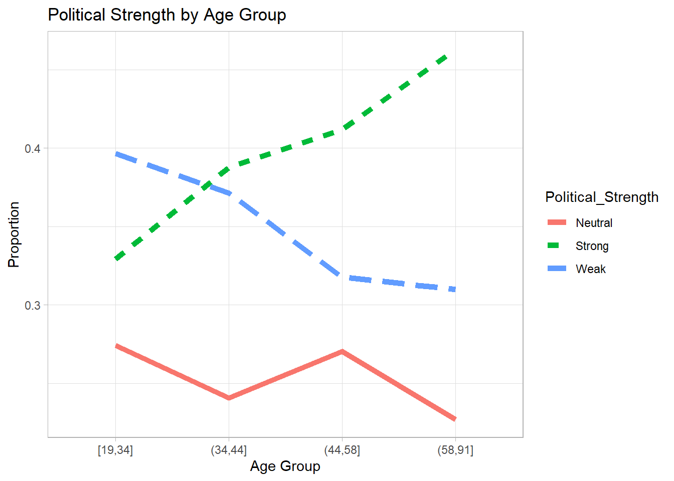
Figure 7.9: Political Strength by Age Group
4. Fit a Multinomial Logistic Model
We model political strength as a function of age and education.
# Fit multinomial logistic regression
Multinomial_Model <-
    multinom(Political_Strength ~ age + educ,
             data = nes96,
             trace = FALSE)
summary(Multinomial_Model)
#> Call:
#> multinom(formula = Political_Strength ~ age + educ, data = nes96,
#>     trace = FALSE)
#>
#> Coefficients:
#>        (Intercept)          age     educ.L     educ.Q     educ.C      educ^4
#> Strong -0.08788729  0.010700364 -0.1098951 -0.2016197 -0.1757739 -0.02116307
#> Weak    0.51976285 -0.004868771 -0.1431104 -0.2405395 -0.2411795  0.18353634
#>            educ^5     educ^6
#> Strong -0.1664377 -0.1359449
#> Weak   -0.1489030 -0.2173144
#>
#> Std. Errors:
#>        (Intercept)         age    educ.L    educ.Q    educ.C    educ^4
#> Strong   0.3017034 0.005280743 0.4586041 0.4318830 0.3628837 0.2964776
#> Weak     0.3097923 0.005537561 0.4920736 0.4616446 0.3881003 0.3169149
#>           educ^5    educ^6
#> Strong 0.2515012 0.2166774
#> Weak   0.2643747 0.2199186
#>
#> Residual Deviance: 2024.596
#> AIC: 2056.596
5. Stepwise Model Selection Based on AIC
We perform stepwise selection to find the best model.
Multinomial_Step <- step(Multinomial_Model, trace = 0)
#> trying - age
#> trying - educ
#> trying - age
Multinomial_Step
#> Call:
#> multinom(formula = Political_Strength ~ age, data = nes96, trace = FALSE)
#>
#> Coefficients:
#>        (Intercept)          age
#> Strong -0.01988977  0.009832916
#> Weak    0.59497046 -0.005954348
#>
#> Residual Deviance: 2030.756
#> AIC: 2038.756
Compare the best model to the full model based on deviance:
pchisq(
    q = deviance(Multinomial_Step) - deviance(Multinomial_Model),
    df = Multinomial_Model$edf - Multinomial_Step$edf,
    lower.tail = FALSE
)
#> [1] 0.9078172
A non-significant p-value suggests no major difference between the full and stepwise models.
6. Predictions & Visualization
Predicting Political Strength Probabilities by Age
# Create data for prediction
PlotData <- data.frame(age = seq(from = 19, to = 91))

# Get predicted probabilities
Preds <- PlotData %>%
    bind_cols(data.frame(predict(Multinomial_Step,
                                 PlotData,
                                 type = "probs")))
# Plot predicted probabilities across age
plot(
    x = Preds$age,
    y = Preds$Neutral,
    type = "l",
    ylim = c(0.2, 0.6),
    col = "black",
    ylab = "Proportion",
    xlab = "Age"
)

lines(x = Preds$age,
      y = Preds$Weak,
      col = "blue")
lines(x = Preds$age,
      y = Preds$Strong,
      col = "red")

legend(
    "topleft",
    legend = c("Neutral", "Weak", "Strong"),
    col = c("black", "blue", "red"),
    lty = 1
)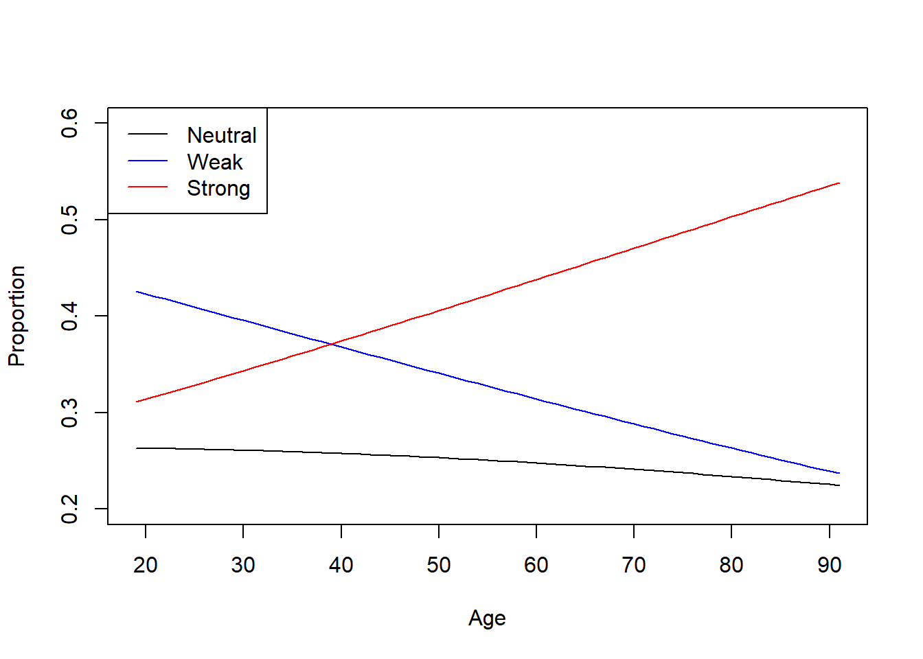
Figure 7.10: Age Group by Predicted Probabilities
Predict for Specific Ages
# Predict class for a 34-year-old
predict(Multinomial_Step, data.frame(age = 34))
#> [1] Weak
#> Levels: Neutral Strong Weak

# Predict probabilities for 34 and 35-year-olds
predict(Multinomial_Step,
        data.frame(age = c(34, 35)),
        type = "probs")
#>     Neutral    Strong      Weak
#> 1 0.2597275 0.3556910 0.3845815
#> 2 0.2594080 0.3587639 0.3818281
7.7.8 Application: Gamma Regression
When response variables are strictly positive, we use Gamma regression.
1. Load and Prepare Data
library(agridat)  # Agricultural dataset
library(ggplot2)

# Load and filter data
dat <- agridat::streibig.competition
gammaDat <- subset(dat, sseeds < 1)  # Keep only barley
gammaDat <-
    transform(gammaDat,
              x = bseeds,
              y = bdwt,
              block = factor(block))
2. Visualization of Inverse Yield
ggplot(gammaDat, aes(x = x, y = 1 / y)) +
    geom_point(aes(color = block, shape = block)) +
    labs(title = "Inverse Yield vs Seeding Rate",
         x = "Seeding Rate",
         y = "Inverse Yield")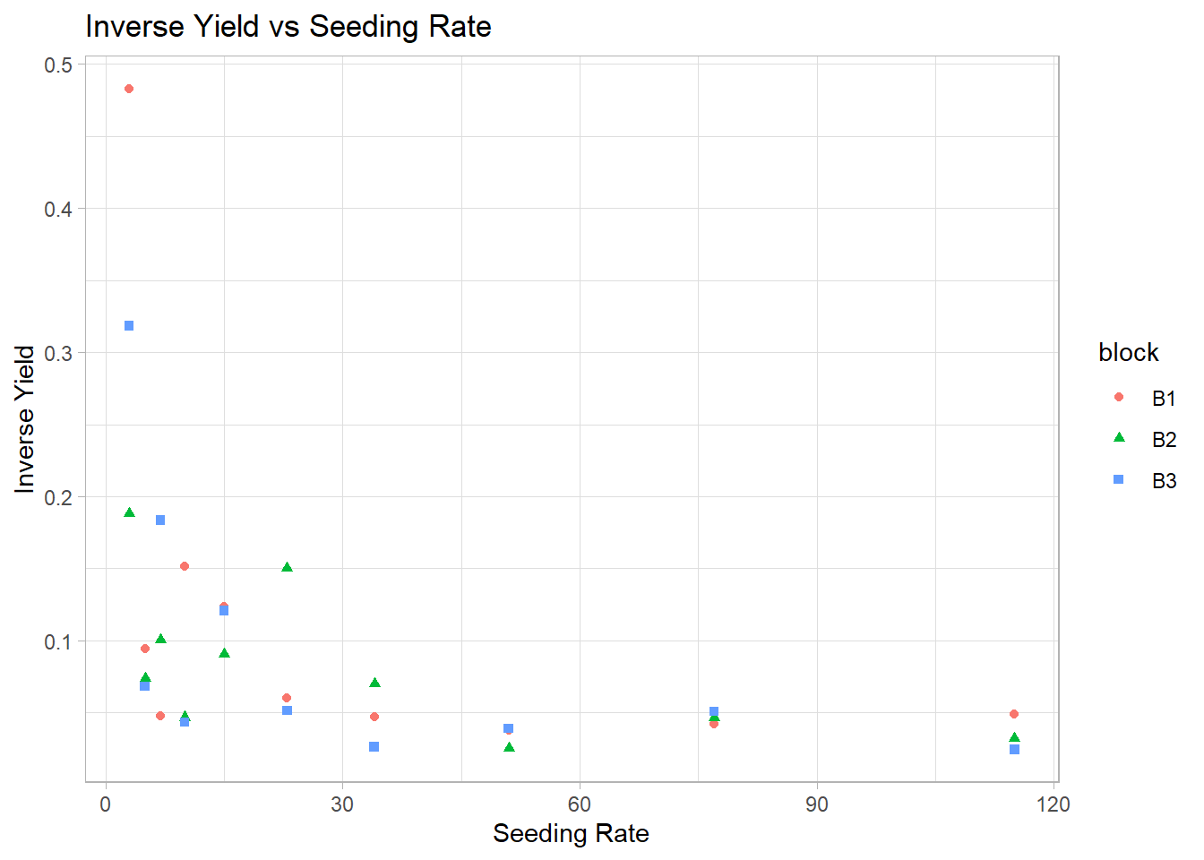
Figure 7.11: Inverse Yield vs Seeding Rate
3. Fit Gamma Regression Model
Gamma regression models yield as a function of seeding rate using an inverse link:
\[ \eta_{ij} = \beta_{0j} + \beta_{1j} x_{ij} + \beta_2 x_{ij}^2, \quad Y_{ij} = \eta_{ij}^{-1} \]
m1 <- glm(y ~ block + block * x + block * I(x^2),
          data = gammaDat, family = Gamma(link = "inverse"))

summary(m1)
#>
#> Call:
#> glm(formula = y ~ block + block * x + block * I(x^2), family = Gamma(link = "inverse"),
#>     data = gammaDat)
#>
#> Coefficients:
#>                  Estimate Std. Error t value Pr(>|t|)
#> (Intercept)     1.115e-01  2.870e-02   3.886 0.000854 ***
#> blockB2        -1.208e-02  3.880e-02  -0.311 0.758630
#> blockB3        -2.386e-02  3.683e-02  -0.648 0.524029
#> x              -2.075e-03  1.099e-03  -1.888 0.072884 .
#> I(x^2)          1.372e-05  9.109e-06   1.506 0.146849
#> blockB2:x       5.198e-04  1.468e-03   0.354 0.726814
#> blockB3:x       7.475e-04  1.393e-03   0.537 0.597103
#> blockB2:I(x^2) -5.076e-06  1.184e-05  -0.429 0.672475
#> blockB3:I(x^2) -6.651e-06  1.123e-05  -0.592 0.560012
#> ---
#> Signif. codes:  0 '***' 0.001 '**' 0.01 '*' 0.05 '.' 0.1 ' ' 1
#>
#> (Dispersion parameter for Gamma family taken to be 0.3232083)
#>
#>     Null deviance: 13.1677  on 29  degrees of freedom
#> Residual deviance:  7.8605  on 21  degrees of freedom
#> AIC: 225.32
#>
#> Number of Fisher Scoring iterations: 5
4. Predictions and Visualization
# Generate new data for prediction
newdf <-
    expand.grid(x = seq(0, 120, length = 50),
                block = factor(c("B1", "B2", "B3")))

# Predict responses
newdf$pred <- predict(m1, newdata = newdf, type = "response")
# Plot predictions
ggplot(gammaDat, aes(x = x, y = y)) +
    geom_point(aes(color = block, shape = block)) +
    geom_line(data = newdf, aes(
        x = x,
        y = pred,
        color = block,
        linetype = block
    )) +
    labs(title = "Predicted Yield by Seeding Rate",
         x = "Seeding Rate",
         y = "Yield")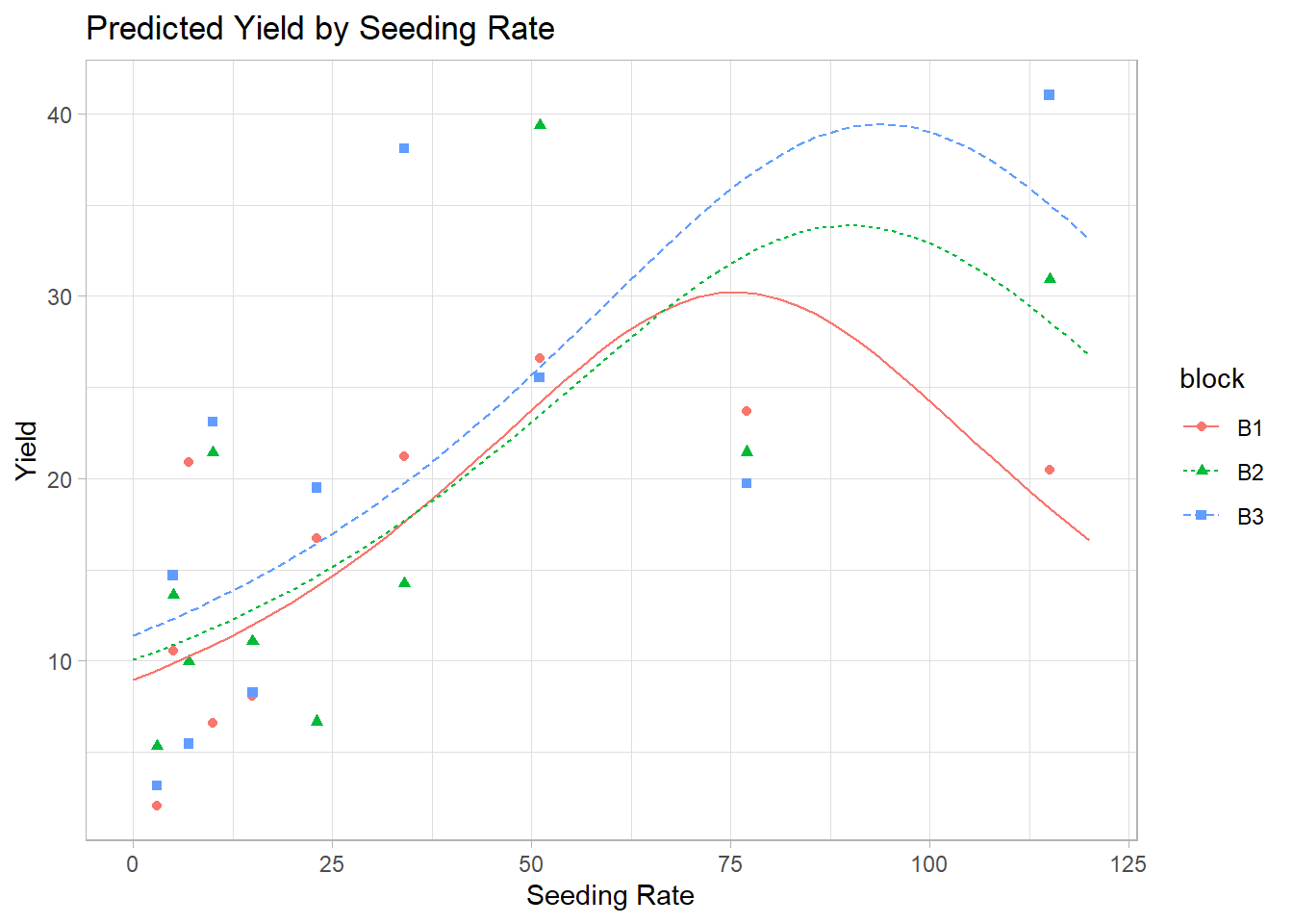
Figure 7.12: Predicted Yield by Seeding Rate
7.8 Generalization of Generalized Linear Models
We have seen that Poisson regression bears similarities to logistic regression. This insight leads us to a broader class of models known as Generalized Linear Models, introduced by Nelder and Wedderburn (1972). These models provide a unified framework for handling different types of response variables while maintaining the fundamental principles of linear modeling.
7.8.1 Exponential Family
The foundation of GLMs is built on the exponential family of distributions, which provides a flexible class of probability distributions that share a common form:
\[ f(y;\theta, \phi) = \exp\left(\frac{\theta y - b(\theta)}{a(\phi)} + c(y, \phi)\right) \]
where:
- \(\theta\) is the natural parameter (canonical parameter),
- \(\phi\) is the dispersion parameter,
- \(a(\phi)\), \(b(\theta)\), and \(c(y, \phi)\) are functions ensuring the proper distributional form.
Distributions in the Exponential Family that Can Be Used in GLMs:
Inverse Gaussian Distribution
Negative Binomial Distribution (used in GLMs but requires overdispersion adjustments)
Multinomial Distribution (for categorical response)
Exponential Family Distributions Not Commonly Used in GLMs:
Beta Distribution
Dirichlet Distribution
Wishart Distribution
Exponential Distribution (can be used indirectly through survival models)
Example: Normal Distribution
Consider a normally distributed response variable \(Y \sim N(\mu, \sigma^2)\). The probability density function (PDF) is:
\[ \begin{aligned} f(y; \mu, \sigma^2) &= \frac{1}{\sqrt{2\pi \sigma^2}} \exp\left(-\frac{(y - \mu)^2}{2\sigma^2}\right) \\ &= \exp\left(-\frac{y^2 - 2y\mu + \mu^2}{2\sigma^2} - \frac{1}{2} \log(2\pi\sigma^2)\right) \end{aligned} \]
Rewriting in exponential family form:
\[ \begin{aligned} f(y; \mu, \sigma^2) &= \exp\left(\frac{y \mu - \frac{\mu^2}{2}}{\sigma^2} - \frac{y^2}{2\sigma^2} - \frac{1}{2} \log(2\pi\sigma^2)\right) \\ &= \exp\left(\frac{\theta y - b(\theta)}{a(\phi)} + c(y, \phi)\right) \end{aligned} \]
where:
- Natural parameter: \(\theta = \mu\)
- Function \(b(\theta)\): \(b(\theta) = \frac{\mu^2}{2}\)
- Dispersion function: \(a(\phi) = \sigma^2 = \phi\)
- Function \(c(y, \phi)\): \(c(y, \phi) = -\frac{1}{2} \left(\frac{y^2}{\phi} + \log(2\pi \sigma^2)\right)\)
7.8.2 Properties of GLM Exponential Families
Expected Value (Mean) \[ E(Y) = b'(\theta) \] where \(b'(\theta) = \frac{\partial b(\theta)}{\partial \theta}\). (Note:
'is “prime,” not transpose).-
Variance \[ \text{Var}(Y) = a(\phi) b''(\theta) = a(\phi) V(\mu) \] where:
- \(V(\mu) = b''(\theta)\) is the variance function, though it only represents the variance when \(a(\phi) = 1\).
If \(a(\phi)\), \(b(\theta)\), and \(c(y, \phi)\) are identifiable, we can derive the expected value and variance of \(Y\).
Examples of Exponential Family Distributions
1. Normal Distribution
For a normal distribution \(Y \sim N(\mu, \sigma^2)\), the exponential family representation is:
\[ f(y; \mu, \sigma^2) = \frac{1}{\sqrt{2\pi \sigma^2}} \exp \left( -\frac{(y - \mu)^2}{2\sigma^2} \right) \]
which can be rewritten in exponential form:
\[ \exp \left( \frac{y\mu - \frac{1}{2} \mu^2}{\sigma^2} - \frac{y^2}{2\sigma^2} - \frac{1}{2} \log(2\pi\sigma^2) \right) \]
From this, we identify:
- \(\theta = \mu\)
- \(b(\theta) = \frac{\theta^2}{2}\)
- \(a(\phi) = \sigma^2\)
Computing derivatives:
\[ b'(\theta) = \frac{\partial b(\theta)}{\partial \theta} = \mu, \quad V(\mu) = b''(\theta) = 1 \]
Thus,
\[ E(Y) = \mu, \quad \text{Var}(Y) = a(\phi) V(\mu) = \sigma^2 \]
2. Poisson Distribution
For a Poisson-distributed response \(Y \sim \text{Poisson}(\mu)\), the probability mass function is:
\[ f(y; \mu) = \frac{\mu^y e^{-\mu}}{y!} \]
Rewriting in exponential form:
\[ \exp(y \log \mu - \mu - \log y!) \]
Thus, we identify:
- \(\theta = \log \mu\)
- \(b(\theta) = e^\theta\)
- \(a(\phi) = 1\)
- \(c(y, \phi) = \log y!\)
Computing derivatives:
\[ E(Y) = b'(\theta) = e^\theta = \mu, \quad \text{Var}(Y) = b''(\theta) = \mu \]
Since \(\mu = E(Y)\), we confirm the variance function:
\[ \text{Var}(Y) = V(\mu) = \mu \]
7.8.3 Structure of a Generalized Linear Model
In a GLM, we model the mean \(\mu\) through a link function that connects it to a linear predictor:
\[ g(\mu) = g(b'(\theta)) = \mathbf{x' \beta} \]
Equivalently,
\[ \mu = g^{-1}(\mathbf{x' \beta}) \]
where:
- \(g(\cdot)\) is the link function, which ensures a transformation between the expected response \(E(Y) = \mu\) and the linear predictor.
- \(\eta = \mathbf{x' \beta}\) is called the linear predictor.
7.8.4 Components of a GLM
A GLM consists of two main components:
7.8.4.1 Random Component
This describes the distribution of the response variable \(Y_1, \dots, Y_n\). The response variables are assumed to follow a distribution from the exponential family, which can be written as:
\[ f(y_i ; \theta_i, \phi) = \exp \left( \frac{\theta_i y_i - b(\theta_i)}{a(\phi)} + c(y_i, \phi) \right) \]
where:
\(Y_i\) are independent random variables.
The canonical parameter \(\theta_i\) may differ for each observation.
The dispersion parameter \(\phi\) is assumed to be constant across all \(i\).
-
The mean response is given by:
\[ \mu_i = E(Y_i) \]
7.8.4.2 Systematic Component
This specifies how the mean response \(\mu\) is related to the explanatory variables \(\mathbf{x}\) through a linear predictor \(\eta\):
-
The systematic component consists of:
- A link function \(g(\mu)\).
- A linear predictor \(\eta = \mathbf{x' \beta}\).
-
Notation:
-
We assume:
\[ g(\mu_i) = \mathbf{x' \beta} = \eta_i \]
The parameter vector \(\mathbf{\beta} = (\beta_1, \dots, \beta_p)'\) needs to be estimated.
-
7.8.5 Canonical Link
In a GLM, a link function \(g(\cdot)\) relates the mean \(\mu_i\) of the response \(Y_i\) to the linear predictor \(\eta_i\) via
\[ \eta_i = g(\mu_i). \]
A canonical link is a special case of \(g(\cdot)\) where
\[ g(\mu_i) = \eta_i = \theta_i, \]
and \(\theta_i\) is the natural parameter of the exponential family. In other words, the link function directly equates the linear predictor \(\eta_i\) with the distribution’s natural parameter \(\theta_i\). Hence, \(g(\mu)\) is canonical if \(g(\mu) = \theta\).
Exponential Family Components
- \(b(\theta)\): the cumulant (moment generating) function, which defines the variance function.
-
\(g(\mu)\): the link function, which must be
- Monotonically increasing
- Continuously differentiable
- Invertible
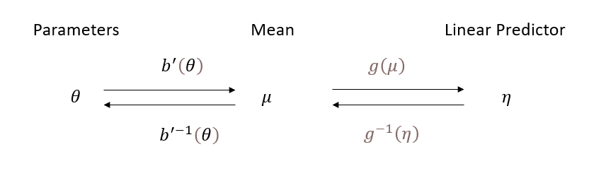
Figure 7.13: GLM Structure
For an exponential-family distribution, the function \(b(\theta)\) is called the cumulant moment generating function, and it relates \(\theta\) to the mean via its derivative:
\[ \mu = b'(\theta) \quad\Longleftrightarrow\quad \theta = b'^{-1}(\mu). \]
By defining the link so that \(g(\mu) = \theta\), we impose \(\eta_i = \theta_i\), which is why \(g(\cdot)\) is termed canonical in this setting.
When the link is canonical, an equivalent way to express this is
\[ \gamma^{-1} \circ g^{-1} = I, \]
indicating that the inverse link \(g^{-1}(\cdot)\) directly maps the linear predictor (now the natural parameter \(\theta\)) back to \(\mu\) in a way that respects the structure of the exponential family.
Choosing \(g(\cdot)\) to be canonical often simplifies mathematical derivations and computations—especially for parameter estimation—because the linear predictor \(\eta\) and the natural parameter \(\theta\) coincide. Common examples of canonical links include:
- Identity link for the normal (Gaussian) distribution
- Log link for the Poisson distribution
- Logit link for the Bernoulli (binomial) distribution
In each case, setting \(\eta = \theta\) streamlines the relationship between the mean and the linear predictor, making the model both elegant and practically convenient.
7.8.6 Inverse Link Functions
The inverse link function \(g^{-1}(\eta)\) (also called the mean function) transforms the linear predictor \(\eta\) (which can take any real value) into a valid mean response \(\mu\).
Example 1: Normal Distribution (Identity Link)
Random Component: \(Y_i \sim N(\mu_i, \sigma^2)\).
Mean Response: \(\mu_i = \theta_i\).
-
Canonical Link Function:
\[ g(\mu_i) = \mu_i \]
(i.e., the identity function).
Example 2: Binomial Distribution (Logit Link)
Random Component: \(Y_i \sim \text{Binomial}(n_i, p_i)\).
-
Mean Response:
\[ \mu_i = \frac{n_i e^{\theta_i}}{1+e^{\theta_i}} \]
-
Canonical Link Function:
\[ g(\mu_i) = \log \left( \frac{\mu_i}{n_i - \mu_i} \right) \]
(Logit link function).
Example 3: Poisson Distribution (Log Link)
Random Component: \(Y_i \sim \text{Poisson}(\mu_i)\).
-
Mean Response:
\[ \mu_i = e^{\theta_i} \]
-
Canonical Link Function:
\[ g(\mu_i) = \log(\mu_i) \]
(Log link function).
Example 4: Gamma Distribution (Inverse Link)
Random Component: \(Y_i \sim \text{Gamma}(\alpha, \mu_i)\).
-
Mean Response:
\[ \mu_i = -\frac{1}{\theta_i} \]
-
Canonical Link Function:
\[ g(\mu_i) = -\frac{1}{\mu_i} \]
(Inverse link function).
The following table presents common GLM link functions and their corresponding inverse functions.
| Link | \(\eta_i = g(\mu_i)\) | \(\mu_i = g^{-1}(\eta_i)\) |
|---|---|---|
| Identity | \(\mu_i\) | \(\eta_i\) |
| Log | \(\log_e \mu_i\) | \(e^{\eta_i}\) |
| Inverse | \(\mu_i^{-1}\) | \(\eta_i^{-1}\) |
| Inverse-square | \(\mu_i^{-2}\) | \(\eta_i^{-1/2}\) |
| Square-root | \(\sqrt{\mu_i}\) | \(\eta_i^2\) |
| Logit | \(\log_e \left( \frac{\mu_i}{1 - \mu_i} \right)\) | \(\frac{1}{1 + e^{-\eta_i}}\) |
| Probit | \(\Phi^{-1}(\mu_i)\) | \(\Phi(\eta_i)\) |
where
\(\mu_i\) is the expected value of the response.
\(\eta_i\) is the linear predictor.
\(\Phi(\cdot)\) represents the CDF of the standard normal distribution.
7.8.7 Estimation of Parameters in GLMs
The GLM framework extends Linear Regression by allowing for response variables that follow exponential family distributions.
Maximum Likelihood Estimation is used to estimate the parameters of the systematic component (\(\beta\)), providing a consistent and efficient approach. The derivation and computation processes are unified, thanks to the exponential form of the model, which simplifies mathematical treatment and implementation.
However, this unification does not extend to the estimation of the dispersion parameter (\(\phi\)), which requires separate treatment, often involving alternative estimation methods such as moment-based approaches or quasi-likelihood estimation.
In GLMs, the response variable \(Y_i\) follows an exponential family distribution characterized by the density function:
\[ f(y_i ; \theta_i, \phi) = \exp\left(\frac{\theta_i y_i - b(\theta_i)}{a(\phi)} + c(y_i, \phi) \right) \]
where:
- \(\theta_i\) is the canonical parameter.
- \(\phi\) is the dispersion parameter (which may be known or estimated separately).
- \(b(\theta_i)\) determines the mean and variance of \(Y_i\).
- \(a(\phi)\) scales the variance.
- \(c(y_i, \phi)\) ensures proper normalization.
For this family, we obtain:
- Mean of \(Y_i\): \[ E(Y_i) = \mu_i = b'(\theta_i) \]
- Variance of \(Y_i\): \[ \text{Var}(Y_i) = b''(\theta_i) a(\phi) = V(\mu_i)a(\phi) \] where \(V(\mu_i)\) is the variance function.
- Systematic component (link function): \[ g(\mu_i) = \eta_i = \mathbf{x}_i' \beta \]
The function \(g(\cdot)\) is the link function, which connects the expected response \(\mu_i\) to the linear predictor \(\mathbf{x}_i' \beta\).
For a single observation \(Y_i\), the log-likelihood function is:
\[ l_i(\beta, \phi) = \frac{\theta_i y_i - b(\theta_i)}{a(\phi)} + c(y_i, \phi) \]
For \(n\) independent observations, the total log-likelihood is:
\[ l(\beta, \phi) = \sum_{i=1}^n l_i(\beta, \phi) \]
Expanding this,
\[ l(\beta, \phi) = \sum_{i=1}^n \left( \frac{\theta_i y_i - b(\theta_i)}{a(\phi)} + c(y_i, \phi) \right). \]
To estimate \(\beta\), we maximize this log-likelihood function.
7.8.7.1 Estimation of Systematic Component (\(\beta\))
To differentiate \(l(\beta,\phi)\) with respect to \(\beta_j\), we apply the chain rule:
\[ \frac{\partial l_i(\beta,\phi)}{\partial \beta_j} = \underbrace{\frac{\partial l_i(\beta,\phi)}{\partial \theta_i}}_{\text{depends on }(y_i - \mu_i)} \times \underbrace{\frac{\partial \theta_i}{\partial \mu_i}}_{= 1/V(\mu_i)\text{ if canonical link}} \times \underbrace{\frac{\partial \mu_i}{\partial \eta_i}}_{\text{depends on the link}} \times \underbrace{\frac{\partial \eta_i}{\partial \beta_j}}_{= x_{ij}}. \]
Let us see why these four pieces appear:
\(l_i(\beta,\phi)\) depends on \(\theta_i\). So we start by computing \(\frac{\partial l_i}{\partial \theta_i}\).
-
\(\theta_i\) (the “natural parameter” in the exponential family) may in turn be a function of \(\mu_i\).
In canonical‐link GLMs, we often have \(\theta_i = \eta_i\).
In more general‐link GLMs,\(\theta_i\) is still some function of \(\mu_i\).
Hence we need \(\frac{\partial \theta_i}{\partial \mu_i}\).
\(\mu_i\) (the mean) is a function of the linear predictor \(\eta_i\). Typically, \(\eta_i = g(\mu_i)\) implies \(\mu_i = g^{-1}(\eta_i)\). So we need \(\frac{\partial \mu_i}{\partial \eta_i}\).
Finally, \(\eta_i = \mathbf{x}_i^\prime \beta\). So the derivative \(\frac{\partial \eta_i}{\partial \beta_j}\) is simply \(x_{ij}\), the \(j\)‐th component of the covariate vector \(\mathbf{x}_i\).
Let us look at each factor in turn.
First term:
\[ \displaystyle \frac{\partial l_i(\beta,\phi)}{\partial \theta_i} \]
Recall
\[ l_i(\theta_i,\phi) = \frac{\theta_i y_i - b(\theta_i)}{a(\phi)} + c(y_i,\phi). \]
- Differentiate \(\theta_i y_i - b(\theta_i)\) with respect to \(\theta_i\): \[
\frac{\partial}{\partial \theta_i} \left[\theta_iy_i - b(\theta_i)\right] = y_i - b'(\theta_i).
\] But by exponential‐family definitions,\(b'(\theta_i) = \mu_i\).
So that is \(y_i - \mu_i\). - Since everything is divided by \(a(\phi)\), we get \[ \frac{\partial l_i}{\partial \theta_i} = \frac{1}{a(\phi)}[y_i - \mu_i]. \] Hence, \[ \boxed{ \frac{\partial l_i(\beta,\phi)}{\partial \theta_i} = \frac{y_i - \mu_i}{a(\phi)}. } \]
Second term: \[ \displaystyle \frac{\partial \theta_i}{\partial \mu_i} \] 1. In an exponential family with canonical link, we have \[ \theta_i = \eta_i = \mathbf{x}_i^\prime \beta. \] Then \(\theta_i\) is actually the same as \(\eta_i\), which is the same as \(g(\mu_i)\). Recall also that if \(\mu_i = b'(\theta_i)\), then \(d\mu_i/d\theta_i = b''(\theta_i)\). But \(b''(\theta_i) = V(\mu_i)\). Hence \[ \frac{d \mu_i}{d \theta_i} = V(\mu_i) \quad\Longrightarrow\quad \frac{d \theta_i}{d \mu_i} = \frac{1}{V(\mu_i)}. \] This identity is a well‐known property of canonical links in the exponential family.
- In more general (non‐canonical) links, \(\theta_i\) may be some other smooth function of \(\mu_i\). The key idea is: if \(\mu_i = b'(\theta_i)\) but \(\eta_i \neq \theta_i\), you would have to carefully derive \(\partial \theta_i / \partial \mu_i\). Often, a canonical link is assumed to keep expressions simpler.
If we assume a canonical link throughout, then
\[ \boxed{ \frac{\partial \theta_i}{\partial \mu_i} = \frac{1}{V(\mu_i)}. } \]
Third term:
\[ \displaystyle \frac{\partial \mu_i}{\partial \eta_i} \]
Here we consider the link function \(g(\cdot)\), defined by
\[ \eta_i = g(\mu_i) \quad\Longrightarrow\quad \mu_i = g^{-1}(\eta_i). \]
For example,
- In a Bernoulli (logistic‐regression) model, \(μg(\mu) = \log\frac{\mu}{1-\mu}\). So \(\mu = g^{-1}(\eta) = \frac{1}{1+e^{-\eta}}\). Then \(\frac{d\mu}{d\eta} = \mu(1-\mu)\).
- For a Poisson (log) link, \(g(\mu) = \log(\mu)\). So \(\mu = e^\eta\). Then \(\frac{d\mu}{d\eta} = e^\eta = \mu\).
- For an identity link, \(g(\mu) = \mu\). Then \(\eta = \mu\) and \(\frac{d\mu}{d\eta} = 1\).
In general,
\[ \boxed{ \frac{\partial \mu_i}{\partial \eta_i} = \left.\frac{d}{d\eta}\left[g^{-1}(\eta)\right]\right|_{\eta=\eta_i} = \left(g^{-1}\right)'(\eta_i). } \]
If the link is also canonical, then typically \(\frac{\partial \mu_i}{\partial \eta_i} = V(\mu_i)\). Indeed, that is consistent with the second term result.
Fourth term:
\[ \displaystyle \frac{\partial \eta_i}{\partial \beta_j} \]
Finally, the linear predictor is
\[ \eta_i = \mathbf{x}_i^\prime \beta = \sum_{k=1}^p x_{ik}\beta_k. \]
Hence, the derivative of \(\eta_i\) with respect to \(\beta_j\) is simply
\[ \boxed{ \frac{\partial \eta_i}{\partial \beta_j} = x_{ij}. } \]
Therefore, for the entire log‐likelihood \(l(\beta, \phi) = \sum_{i=1}^n l_i(\beta,\phi)\), we sum over \(i\):
\[ \boxed{ \frac{\partial l(\beta,\phi)}{\partial \beta_j} = \sum_{i=1}^n \left[ \frac{y_i - \mu_i}{a(\phi)} \times \frac{1}{V(\mu_i)} \times \frac{\partial \mu_i}{\partial \eta_i} \times x_{ij} \right] } \]
To simplify expressions, we define the weight:
\[ w_i = \left(\left(\frac{\partial \eta_i}{\partial \mu_i}\right)^2 V(\mu_i)\right)^{-1}. \]
For canonical links, this often simplifies to \(w_i = V(\mu_i)\), such as:
- Bernoulli (logit link): \(w_i = p_i(1-p_i)\).
- Poisson (log link): \(w_i = \mu_i\).
Rewriting the score function in terms of \(w_i\):
\[ \frac{\partial l(\beta,\phi)}{\partial \beta_j} = \sum_{i=1}^n \left[ \frac{y_i - \mu_i}{a(\phi)} \times w_i \times \frac{\partial \eta_i}{\partial \mu_i} \times x_{ij} \right]. \]
To use the Newton-Raphson Algorithm for estimating \(\beta\), we require the expected second derivative:
\[ - E\left(\frac{\partial^2 l(\beta,\phi)}{\partial \beta_j \partial \beta_k}\right), \]
which corresponds to the \((j,k)\)-th element of the Fisher information matrix \(\mathbf{I}(\beta)\):
\[ \mathbf{I}_{jk}(\beta) = - E\left(\frac{\partial^2 l(\beta,\phi)}{\partial \beta_j \partial \beta_k}\right) = \sum_{i=1}^n \frac{w_i}{a(\phi)}x_{ij}x_{ik}. \]
Example: Bernoulli Model with Logit Link
For a Bernoulli response with a logit link function (canonical link), we have:
\[ \begin{aligned} b(\theta) &= \log(1 + \exp(\theta)) = \log(1 + \exp(\mathbf{x'}\beta)), \\ a(\phi) &= 1, \\ c(y_i, \phi) &= 0. \end{aligned} \]
From the mean and link function:
\[ \begin{aligned} E(Y) = b'(\theta) &= \frac{\exp(\theta)}{1 + \exp(\theta)} = \mu = p, \\ \eta = g(\mu) &= \log\left(\frac{\mu}{1-\mu}\right) = \theta = \log\left(\frac{p}{1-p}\right) = \mathbf{x'}\beta. \end{aligned} \]
The log-likelihood for \(Y_i\) is:
\[ l_i (\beta, \phi) = \frac{y_i \theta_i - b(\theta_i)}{a(\phi)} + c(y_i, \phi) = y_i \mathbf{x'}_i \beta - \log(1+ \exp(\mathbf{x'}\beta)). \]
We also obtain:
\[ \begin{aligned} V(\mu_i) &= \mu_i(1-\mu_i) = p_i (1-p_i), \\ \frac{\partial \mu_i}{\partial \eta_i} &= p_i(1-p_i). \end{aligned} \]
Thus, the first derivative simplifies as:
\[ \begin{aligned} \frac{\partial l(\beta, \phi)}{\partial \beta_j} &= \sum_{i=1}^n \left[\frac{y_i - \mu_i}{a(\phi)} \times \frac{1}{V(\mu_i)}\times \frac{\partial \mu_i}{\partial \eta_i} \times x_{ij} \right] \\ &= \sum_{i=1}^n (y_i - p_i) \times \frac{1}{p_i(1-p_i)} \times p_i(1-p_i) \times x_{ij} \\ &= \sum_{i=1}^n (y_i - p_i) x_{ij} \\ &= \sum_{i=1}^n \left(y_i - \frac{\exp(\mathbf{x'}_i\beta)}{1+ \exp(\mathbf{x'}_i\beta)}\right)x_{ij}. \end{aligned} \]
The weight term in this case is:
\[ w_i = \left(\left(\frac{\partial \eta_i}{\partial \mu_i} \right)^2 V(\mu_i)\right)^{-1} = p_i (1-p_i). \]
Thus, the Fisher information matrix has elements:
\[ \mathbf{I}_{jk}(\beta) = \sum_{i=1}^n \frac{w_i}{a(\phi)} x_{ij}x_{ik} = \sum_{i=1}^n p_i (1-p_i)x_{ij}x_{ik}. \]`
The Fisher-Scoring algorithm for the Maximum Likelihood estimate of \(\mathbf{\beta}\) is given by:
\[ \left( \begin{array} {c} \beta_1 \\ \beta_2 \\ \vdots \\ \beta_p \\ \end{array} \right)^{(m+1)} = \left( \begin{array} {c} \beta_1 \\ \beta_2 \\ \vdots \\ \beta_p \\ \end{array} \right)^{(m)} + \mathbf{I}^{-1}(\mathbf{\beta}) \left( \begin{array} {c} \frac{\partial l (\beta, \phi)}{\partial \beta_1} \\ \frac{\partial l (\beta, \phi)}{\partial \beta_2} \\ \vdots \\ \frac{\partial l (\beta, \phi)}{\partial \beta_p} \\ \end{array} \right)\Bigg|_{\beta = \beta^{(m)}} \]
This is similar to the Newton-Raphson Algorithm, except that we replace the observed matrix of second derivatives (Hessian) with its expected value.
In matrix representation, the score function (gradient of the log-likelihood) is:
\[ \begin{aligned} \frac{\partial l }{\partial \beta} &= \frac{1}{a(\phi)}\mathbf{X'W\Delta(y - \mu)} \\ &= \frac{1}{a(\phi)}\mathbf{F'V^{-1}(y - \mu)} \end{aligned} \]
The expected Fisher information matrix is:
\[ \mathbf{I}(\beta) = \frac{1}{a(\phi)}\mathbf{X'WX} = \frac{1}{a(\phi)}\mathbf{F'V^{-1}F} \]
where:
- \(\mathbf{X}\) is an \(n \times p\) matrix of covariates.
- \(\mathbf{W}\) is an \(n \times n\) diagonal matrix with \((i,i)\)-th element given by \(w_i\).
- \(\mathbf{\Delta}\) is an \(n \times n\) diagonal matrix with \((i,i)\)-th element given by \(\frac{\partial \eta_i}{\partial \mu_i}\).
- \(\mathbf{F} = \frac{\partial \mu}{\partial \beta}\) is an \(n \times p\) matrix, where the \(i\)-th row is given by \(\frac{\partial \mu_i}{\partial \beta} = (\frac{\partial \mu_i}{\partial \eta_i})\mathbf{x}'_i\).
- \(\mathbf{V}\) is an \(n \times n\) diagonal matrix with \((i,i)\)-th element given by \(V(\mu_i)\).
Setting the derivative of the log-likelihood equal to zero gives the MLE equations:
\[ \mathbf{F'V^{-1}y} = \mathbf{F'V^{-1}\mu} \]
Since all components of this equation (except for \(\mathbf{y}\)) depend on \(\beta\), we solve iteratively.
Special Cases
- Canonical Link Function
If a canonical link is used, the estimating equations simplify to:
\[ \mathbf{X'y} = \mathbf{X'\mu} \]
- Identity Link Function
If the identity link is used, the estimating equation reduces to:
\[ \mathbf{X'V^{-1}y} = \mathbf{X'V^{-1}X\hat{\beta}} \]
which leads to the Generalized Least Squares estimator:
\[ \hat{\beta} = (\mathbf{X'V^{-1}X})^{-1} \mathbf{X'V^{-1}y} \]
Fisher-Scoring Algorithm in General Form
The iterative update formula for Fisher-scoring can be rewritten as:
\[ \beta^{(m+1)} = \beta^{(m)} + \mathbf{(\hat{F}'\hat{V}^{-1}\hat{F})^{-1}\hat{F}'\hat{V}^{-1}(y- \hat{\mu})} \]
Since \(\hat{F}, \hat{V}, \hat{\mu}\) depend on \(\beta\), we evaluate them at \(\beta^{(m)}\).
From an initial guess \(\beta^{(0)}\), we iterate until convergence.
Notes:
- If \(a(\phi)\) is a constant or takes the form \(m_i \phi\) with known \(m_i\), then \(\phi\) cancels from the equations, simplifying the estimation.
7.8.7.2 Estimation of Dispersion Parameter (\(\phi\))
There are two common approaches to estimating \(\phi\):
- Maximum Likelihood Estimation
The derivative of the log-likelihood with respect to \(\phi\) is:
\[ \frac{\partial l_i}{\partial \phi} = \frac{(\theta_i y_i - b(\theta_i)a'(\phi))}{a^2(\phi)} + \frac{\partial c(y_i,\phi)}{\partial \phi} \]
The MLE of \(\phi\) satisfies the equation:
\[ \frac{a^2(\phi)}{a'(\phi)}\sum_{i=1}^n \frac{\partial c(y_i, \phi)}{\partial \phi} = \sum_{i=1}^n(\theta_i y_i - b(\theta_i)) \]
Challenges:
For distributions other than the normal case, the expression for \(\frac{\partial c(y,\phi)}{\partial \phi}\) is often complicated.
Even with a canonical link function and constant \(a(\phi)\), there is no simple general expression for the expected Fisher information:
\[ -E\left(\frac{\partial^2 l}{\partial \phi^2} \right) \]
This means that the unification GLMs provide for estimating \(\beta\) does not extend as neatly to \(\phi\).
- Moment Estimation (Bias-Corrected \(\chi^2\) Method)
The MLE is not the conventional approach for estimating \(\phi\) in Generalized Linear Models.
-
For an exponential family distribution, the variance function is:
\[ \text{Var}(Y) = V(\mu)a(\phi) \]
This implies the following moment-based estimator:
\[ \begin{aligned} a(\phi) &= \frac{\text{Var}(Y)}{V(\mu)} = \frac{E(Y- \mu)^2}{V(\mu)} \\ a(\hat{\phi}) &= \frac{1}{n-p} \sum_{i=1}^n \frac{(y_i -\hat{\mu}_i)^2}{V(\hat{\mu}_i)} \end{aligned} \]
where \(p\) is the number of parameters in \(\beta\).
-
For a GLM with a canonical link function \(g(.)= (b'(.))^{-1}\):
\[ \begin{aligned} g(\mu) &= \theta = \eta = \mathbf{x'\beta} \\ \mu &= g^{-1}(\eta)= b'(\eta) \end{aligned} \]
Using this, the moment estimator for \(a(\phi) = \phi\) becomes:
\[ \hat{\phi} = \frac{1}{n-p} \sum_{i=1}^n \frac{(y_i - g^{-1}(\hat{\eta}_i))^2}{V(g^{-1}(\hat{\eta}_i))} \]
| Approach | Description | Pros | Cons |
|---|---|---|---|
| MLE | Estimates \(\phi\) by maximizing the likelihood function | Theoretically optimal | Computationally complex, lacks a general closed-form solution |
| Moment Estimation | Uses a bias-corrected \(\chi^2\) method based on residual variance | Simpler, widely used in GLMs | Not as efficient as MLE |
7.8.8 Inference
The estimated variance of \(\hat{\beta}\) is given by:
\[ \hat{\text{var}}(\beta) = a(\phi)(\mathbf{\hat{F}'\hat{V}^{-1}\hat{F}})^{-1} \]
where:
\(\mathbf{V}\) is an \(n \times n\) diagonal matrix with diagonal elements given by \(V(\mu_i)\).
-
\(\mathbf{F}\) is an \(n \times p\) matrix given by:
\[ \mathbf{F} = \frac{\partial \mu}{\partial \beta} \]
Since \(\mathbf{V}\) and \(\mathbf{F}\) depend on the mean \(\mu\) (and thus on \(\beta\)), their estimates \(\mathbf{\hat{V}}\) and \(\mathbf{\hat{F}}\) depend on \(\hat{\beta}\).
To test a general hypothesis:
\[ H_0: \mathbf{L\beta = d} \]
where \(\mathbf{L}\) is a \(q \times p\) matrix, we use the Wald test:
\[ W = \mathbf{(L \hat{\beta}-d)'(a(\phi)L(\hat{F}'\hat{V}^{-1}\hat{F})L')^{-1}(L \hat{\beta}-d)} \]
Under \(H_0\), the Wald statistic follows a chi-square distribution:
\[ W \sim \chi^2_q \]
where \(q\) is the rank of \(\mathbf{L}\).
Special Case: Testing a Single Coefficient
For a hypothesis of the form:
\[ H_0: \beta_j = 0 \]
the Wald test simplifies to:
\[ W = \frac{\hat{\beta}_j^2}{\hat{\text{var}}(\hat{\beta}_j)} \sim \chi^2_1 \]
asymptotically.
Another common test is the likelihood ratio test, which compares the likelihoods of a full model and a reduced model:
\[ \Lambda = 2 \big(l(\hat{\beta}_f) - l(\hat{\beta}_r)\big) \sim \chi^2_q \]
where:
- \(l(\hat{\beta}_f)\) is the log-likelihood of the full model.
- \(l(\hat{\beta}_r)\) is the log-likelihood of the reduced model.
- \(q\) is the number of constraints used in fitting the reduced model.
| Test | Pros | Cons |
|---|---|---|
| Wald Test | Easy to compute, does not require fitting two models | May perform poorly in small samples |
| Likelihood Ratio Test | More accurate, especially for small samples | Requires fitting both full and reduced models |
While the Wald test is more convenient, the likelihood ratio test is often preferred when sample sizes are small, as it tends to have better statistical properties.
7.8.9 Deviance
Deviance plays a crucial role in:
- Goodness-of-fit assessment: Checking how well a model explains the observed data.
- Statistical inference: Used in hypothesis testing, particularly likelihood ratio tests.
- Estimating dispersion parameters: Helps in refining variance estimates.
- Model comparison: Facilitates selection between competing models.
Assuming the dispersion parameter \(\phi\) is known, let:
\(\tilde{\theta}\) be the MLE under the full model.
\(\hat{\theta}\) be the MLE under the reduced model.
The likelihood ratio statistic (twice the difference in log-likelihoods) is:
\[ 2\sum_{i=1}^{n} \frac{y_i (\tilde{\theta}_i- \hat{\theta}_i)-b(\tilde{\theta}_i) + b(\hat{\theta}_i)}{a_i(\phi)} \]
For exponential family distributions, the mean parameter is:
\[ \mu = E(y) = b'(\theta) \]
Thus, the natural parameter is a function of \(\mu\):
\[ \theta = \theta(\mu) = b'^{-1}(\mu) \]
Rewriting the likelihood ratio statistic in terms of \(\mu\):
\[ 2 \sum_{i=1}^n \frac{y_i\{\theta(\tilde{\mu}_i) - \theta(\hat{\mu}_i)\} - b(\theta(\tilde{\mu}_i)) + b(\theta(\hat{\mu}_i))}{a_i(\phi)} \]
A saturated model provides the fullest possible fit, where each observation is perfectly predicted:
\[ \tilde{\mu}_i = y_i, \quad i = 1, \dots, n \]
Setting \(\tilde{\theta}_i^* = \theta(y_i)\) and \(\hat{\theta}_i^* = \theta (\hat{\mu}_i)\), the likelihood ratio simplifies to:
\[ 2 \sum_{i=1}^{n} \frac{y_i (\tilde{\theta}_i^* - \hat{\theta}_i^*) - b(\tilde{\theta}_i^*) + b(\hat{\theta}_i^*)}{a_i(\phi)} \]
Following McCullagh (2019), for \(a_i(\phi) = \phi\), we define the scaled deviance as:
\[ D^*(\mathbf{y, \hat{\mu}}) = \frac{2}{\phi} \sum_{i=1}^n \{y_i (\tilde{\theta}_i^*- \hat{\theta}_i^*) - b(\tilde{\theta}_i^*) + b(\hat{\theta}_i^*)\} \]
and the deviance as:
\[ D(\mathbf{y, \hat{\mu}}) = \phi D^*(\mathbf{y, \hat{\mu}}) \]
where:
- \(D^*(\mathbf{y, \hat{\mu}})\) is scaled deviance.
- \(D(\mathbf{y, \hat{\mu}})\) is deviance.
In some models, \(a_i(\phi) = \phi m_i\), where \(m_i\) is a known scalar that varies across observations. Then, the scaled deviance is:
\[ D^*(\mathbf{y, \hat{\mu}}) = \sum_{i=1}^n \frac{2\{y_i (\tilde{\theta}_i^*- \hat{\theta}_i^*) - b(\tilde{\theta}_i^*) + b(\hat{\theta}_i^*)\}}{\phi m_i} \]
The deviance is often decomposed into deviance contributions:
\[ D^*(\mathbf{y, \hat{\mu}}) = \sum_{i=1}^n d_i \]
where \(d_i\) is the deviance contribution from the \(i\)-th observation.
Uses of Deviance:
\(D\) is used for model selection.
\(D^*\) is used for goodness-of-fit tests, as it is a likelihood ratio statistic:
\[ D^*(\mathbf{y, \hat{\mu}}) = 2\{l(\mathbf{y,\tilde{\mu}})-l(\mathbf{y,\hat{\mu}})\} \]
- The individual deviance contributions \(d_i\) are used to form deviance residuals.
Deviance for Normal Distribution
For the normal distribution:
\[ \begin{aligned} \theta &= \mu, \\ \phi &= \sigma^2, \\ b(\theta) &= \frac{1}{2} \theta^2, \\ a(\phi) &= \phi. \end{aligned} \]
The MLEs are:
\[ \begin{aligned} \tilde{\theta}_i &= y_i, \\ \hat{\theta}_i &= \hat{\mu}_i = g^{-1}(\hat{\eta}_i). \end{aligned} \]
The deviance simplifies to:
\[ \begin{aligned} D &= 2 \sum_{i=1}^n \left(y_i^2 - y_i \hat{\mu}_i - \frac{1}{2} y_i^2 + \frac{1}{2} \hat{\mu}_i^2 \right) \\ &= \sum_{i=1}^n (y_i^2 - 2y_i \hat{\mu}_i + \hat{\mu}_i^2) \\ &= \sum_{i=1}^n (y_i - \hat{\mu}_i)^2. \end{aligned} \]
Thus, for the normal model, the deviance corresponds to the residual sum of squares.
Deviance for Poisson Distribution
For the Poisson distribution:
\[ \begin{aligned} f(y) &= \exp\{y\log(\mu) - \mu - \log(y!)\}, \\ \theta &= \log(\mu), \\ b(\theta) &= \exp(\theta), \\ a(\phi) &= 1. \end{aligned} \]
MLEs:
\[ \begin{aligned} \tilde{\theta}_i &= \log(y_i), \\ \hat{\theta}_i &= \log(\hat{\mu}_i), \\ \hat{\mu}_i &= g^{-1}(\hat{\eta}_i). \end{aligned} \]
The deviance simplifies to:
\[ \begin{aligned} D &= 2 \sum_{i = 1}^n \left(y_i \log(y_i) - y_i \log(\hat{\mu}_i) - y_i + \hat{\mu}_i \right) \\ &= 2 \sum_{i = 1}^n \left[y_i \log\left(\frac{y_i}{\hat{\mu}_i}\right) - (y_i - \hat{\mu}_i) \right]. \end{aligned} \]
The deviance contribution for each observation:
\[ d_i = 2 \left[y_i \log\left(\frac{y_i}{\hat{\mu}_i}\right) - (y_i - \hat{\mu}_i)\right]. \]
7.8.9.1 Analysis of Deviance
The Analysis of Deviance is a likelihood-based approach for comparing nested models in GLM. It is analogous to the [Analysis of Variance (ANOVA)] in linear models.
When comparing a reduced model (denoted by \(\hat{\mu}_r\)) and a full model (denoted by \(\hat{\mu}_f\)), the difference in scaled deviance follows an asymptotic chi-square distribution:
\[ D^*(\mathbf{y;\hat{\mu}_r}) - D^*(\mathbf{y;\hat{\mu}_f}) = 2\{l(\mathbf{y;\hat{\mu}_f})-l(\mathbf{y;\hat{\mu}_r})\} \sim \chi^2_q \]
where \(q\) is the difference in the number of free parameters between the two models.
This test provides a means to assess whether the additional parameters in the full model significantly improve model fit.
The dispersion parameter \(\phi\) is estimated as:
\[ \hat{\phi} = \frac{D(\mathbf{y, \hat{\mu}})}{n - p} \]
where:
- \(D(\mathbf{y, \hat{\mu}})\) is the deviance of the fitted model.
- \(n\) is the total number of observations.
- \(p\) is the number of estimated parameters.
Caution: The frequent use of \(\chi^2\) tests can be problematic due to their reliance on asymptotic approximations, especially for small samples or overdispersed data (McCullagh 2019).
7.8.9.2 Deviance Residuals
Since deviance plays a role in model evaluation, we define deviance residuals to examine individual data points. Given that the total deviance is:
\[ D = \sum_{i=1}^{n}d_i \]
the deviance residual for observation \(i\) is:
\[ r_{D_i} = \text{sign}(y_i -\hat{\mu}_i)\sqrt{d_i} \]
where:
- \(d_i\) is the deviance contribution from observation \(i\).
- The sign function preserves the direction of the residual.
To account for varying leverage, we define the standardized deviance residual:
\[ r_{s,i} = \frac{y_i -\hat{\mu}_i}{\hat{\sigma}(1-h_{ii})^{1/2}} \]
where:
- \(h_{ii}\) is the leverage of observation \(i\).
- \(\hat{\sigma}\) is an estimate of the standard deviation.
Alternatively, using the GLM hat matrix:
\[ \mathbf{H}^{GLM} = \mathbf{W}^{1/2}X(X'WX)^{-1}X'\mathbf{W}^{-1/2} \]
where \(\mathbf{W}\) is an \(n \times n\) diagonal matrix with \((i,i)\)-th element given by \(w_i\) (see Estimation of Systematic Component (\(\beta\))), we express standardized deviance residuals as:
\[ r_{s, D_i} = \frac{r_{D_i}}{\{\hat{\phi}(1-h_{ii}^{glm})\}^{1/2}} \]
where \(h_{ii}^{glm}\) is the \(i\)-th diagonal element of \(\mathbf{H}^{GLM}\).
7.8.9.3 Pearson Chi-Square Residuals
Another goodness-of-fit statistic is the Pearson Chi-Square statistic, defined as:
\[ X^2 = \sum_{i=1}^{n} \frac{(y_i - \hat{\mu}_i)^2}{V(\hat{\mu}_i)} \]
where:
- \(\hat{\mu}_i\) is the fitted mean response.
- \(V(\hat{\mu}_i)\) is the variance function of the response.
The Scaled Pearson \(\chi^2\) statistic is:
\[ \frac{X^2}{\phi} \sim \chi^2_{n-p} \]
where \(p\) is the number of estimated parameters.
The Pearson residuals are:
\[ X^2_i = \frac{(y_i - \hat{\mu}_i)^2}{V(\hat{\mu}_i)} \]
These residuals assess the difference between observed and fitted values, standardized by the variance.
If the assumptions hold:
Independent samples
-
No overdispersion: If \(\phi = 1\), we expect:
\[ \frac{D(\mathbf{y;\hat{\mu}})}{n-p} \approx 1, \quad \frac{X^2}{n-p} \approx 1 \]
A value substantially greater than 1 suggests overdispersion or model misspecification.
Multiple groups: If the model includes categorical predictors, separate calculations may be needed for each group.
Under these assumptions, both:
\[ \frac{X^2}{\phi} \quad \text{and} \quad D^*(\mathbf{y; \hat{\mu}}) \]
follow a \(\chi^2_{n-p}\) distribution.
set.seed(123)
n <- 100
x <- rnorm(n)
y <- rpois(n, lambda = exp(0.5 + 0.3 * x))

# Poisson response
# Fit Poisson GLM
fit <- glm(y ~ x, family = poisson(link = "log"))

# Extract deviance and Pearson residuals
deviance_residuals <- residuals(fit, type = "deviance")
pearson_residuals  <- residuals(fit, type = "pearson")
# Display residual summaries
summary(deviance_residuals)
#>    Min. 1st Qu.  Median    Mean 3rd Qu.    Max.
#> -2.1286 -1.0189 -0.1441 -0.1806  0.6171  1.8942
summary(pearson_residuals)
#>      Min.   1st Qu.    Median      Mean   3rd Qu.      Max.
#> -1.505136 -0.837798 -0.140873  0.002003  0.658076  2.366618
The residuals suggest a reasonably well-fitted model with a slight underprediction tendency.
No extreme deviations or severe skewness.
The largest residuals indicate potential outliers, but they are not extreme enough to immediately suggest model inadequacy.
7.8.10 Diagnostic Plots
Standardized residual plots help diagnose potential issues with model specification, such as an incorrect link function or variance structure. Common residual plots include:
Plot of Standardized Deviance Residuals vs. Fitted Values
\[ \text{plot}(r_{s, D_i}, \hat{\mu}_i) \] or
\[ \text{plot}(r_{s, D_i}, T(\hat{\mu}_i)) \] where \(T(\hat{\mu}_i)\) is a constant information scale transformation, which adjusts \(\hat{\mu}_i\) to maintain a stable variance across observations.Plot of Standardized Deviance Residuals vs. Linear Predictor
\[ \text{plot}(r_{s, D_i}, \hat{\eta}_i) \] where \(\hat{\eta}_i\) represents the linear predictor before applying the link function.
The following table summarizes the commonly used transformations \(T(\hat{\mu}_i)\) for different random components:
| Random Component | \(T(\hat{\mu}_i)\) |
|---|---|
| Normal | \(\hat{\mu}\) |
| Poisson | \(2\sqrt{\hat{\mu}}\) |
| Binomial | \(2 \sin^{-1}(\sqrt{\hat{\mu}})\) |
| Gamma | \(2 \log(\hat{\mu})\) |
| Inverse Gaussian | \(-2\hat{\mu}^{-1/2}\) |
Interpretation of Residual Plots
- Trend in residuals: Indicates an incorrect link function or an inappropriate scale transformation.
- Systematic change in residual range with \(T(\hat{\mu})\): Suggests an incorrect choice of random component—i.e., the assumed variance function does not match the data.
- Plot of absolute residuals vs. fitted values:
\[ \text{plot}(|r_{D_i}|, \hat{\mu}_i) \] This checks whether the variance function is correctly specified.
7.8.11 Goodness of Fit
To assess how well the model fits the data, we use:
For nested models, likelihood-based information criteria provide a comparison metric:
\[ \begin{aligned} AIC &= -2l(\mathbf{\hat{\mu}}) + 2p \\ AICC &= -2l(\mathbf{\hat{\mu}}) + 2p \left(\frac{n}{n-p-1} \right) \\ BIC &= -2l(\mathbf{\hat{\mu}}) + p \log(n) \end{aligned} \]
where:
- \(l(\hat{\mu})\) is the log-likelihood at the estimated parameters.
- \(p\) is the number of model parameters.
- \(n\) is the number of observations.
Important Considerations:
The same data and model structure (i.e., same link function and assumed random component distribution) must be used for comparisons.
Models can differ in number of parameters but must remain consistent in other respects.
While traditional \(R^2\) is not directly applicable to GLMs, an analogous measure is:
\[ R^2_p = 1 - \frac{l(\hat{\mu})}{l(\hat{\mu}_0)} \]
where \(l(\hat{\mu}_0)\) is the log-likelihood of a model with only an intercept.
For binary response models, a rescaled generalized \(R^2\) is often used:
\[ \bar{R}^2 = \frac{R^2_*}{\max(R^2_*)} = \frac{1-\exp\left(-\frac{2}{n}(l(\hat{\mu}) - l(\hat{\mu}_0))\right)}{1 - \exp\left(\frac{2}{n} l(\hat{\mu}_0) \right)} \]
where the denominator ensures the maximum possible \(R^2\) scaling.
7.8.12 Over-Dispersion
Over-dispersion occurs when the observed variance exceeds what the assumed model allows. This is common in Poisson and Binomial models.
Variance Assumptions for Common Random Components
| Random Component | Standard Assumption (\(\text{var}(Y)\)) | Alternative Model Allowing Over-Dispersion (\(V(\mu)\)) |
|---|---|---|
| Binomial | \(n \mu (1- \mu)\) | \(\phi n \mu (1- \mu)\), where \(m_i = n\) |
| Poisson | \(\mu\) | \(\phi \mu\) |
- By default, \(\phi = 1\), meaning the variance follows the assumed model.
- If \(\phi \neq 1\), the variance differs from the expectation:
- \(\phi > 1\): Over-dispersion (greater variance than expected).
- \(\phi < 1\): Under-dispersion (less variance than expected).
This discrepancy suggests the assumed random component distribution may be inappropriate.
To account for dispersion issues, we can:
-
Choose a more flexible random component distribution
- Negative Binomial for over-dispersed Poisson data.
- Conway-Maxwell Poisson for both over- and under-dispersed count data.
-
Use Mixed Models to account for random effects
- Nonlinear and Generalized Linear Mixed Models introduce random effects, which can help capture additional variance.
# Load necessary libraries
library(ggplot2)
library(MASS)   # For negative binomial models
library(MuMIn)  # For R^2 in GLMs
library(glmmTMB) # For handling overdispersion

# Generate Example Data
set.seed(123)
n <- 100
x <- rnorm(n)
mu <- exp(0.5 + 0.3 * x)  # True mean function
y <- rpois(n, lambda = mu)  # Poisson outcome

# Fit a Poisson GLM
model_pois <- glm(y ~ x, family = poisson(link = "log"))

# Compute residuals
resid_dev <- residuals(model_pois, type = "deviance")
fitted_vals <- fitted(model_pois)
# Standardized Residual Plot: Residuals vs Fitted Values
ggplot(data = data.frame(fitted_vals, resid_dev),
       aes(x = fitted_vals, y = resid_dev)) +
    geom_point(alpha = 0.6) +
    geom_smooth(method = "loess",
                color = "red",
                se = FALSE) +
    theme_minimal() +
    labs(title = "Standardized Deviance Residuals vs Fitted Values",
         x = "Fitted Values", y = "Standardized Deviance Residuals")
Figure 7.14: Standardized Deviance Residuals vs Fitted Values
# Absolute Residuals vs Fitted Values (Variance Function Check)
ggplot(data = data.frame(fitted_vals, abs_resid = abs(resid_dev)),
       aes(x = fitted_vals, y = abs_resid)) +
    geom_point(alpha = 0.6) +
    geom_smooth(method = "loess",
                color = "blue",
                se = FALSE) +
    theme_minimal() +
    labs(title = "Absolute Deviance Residuals vs Fitted Values",
         x = "Fitted Values", y = "|Residuals|")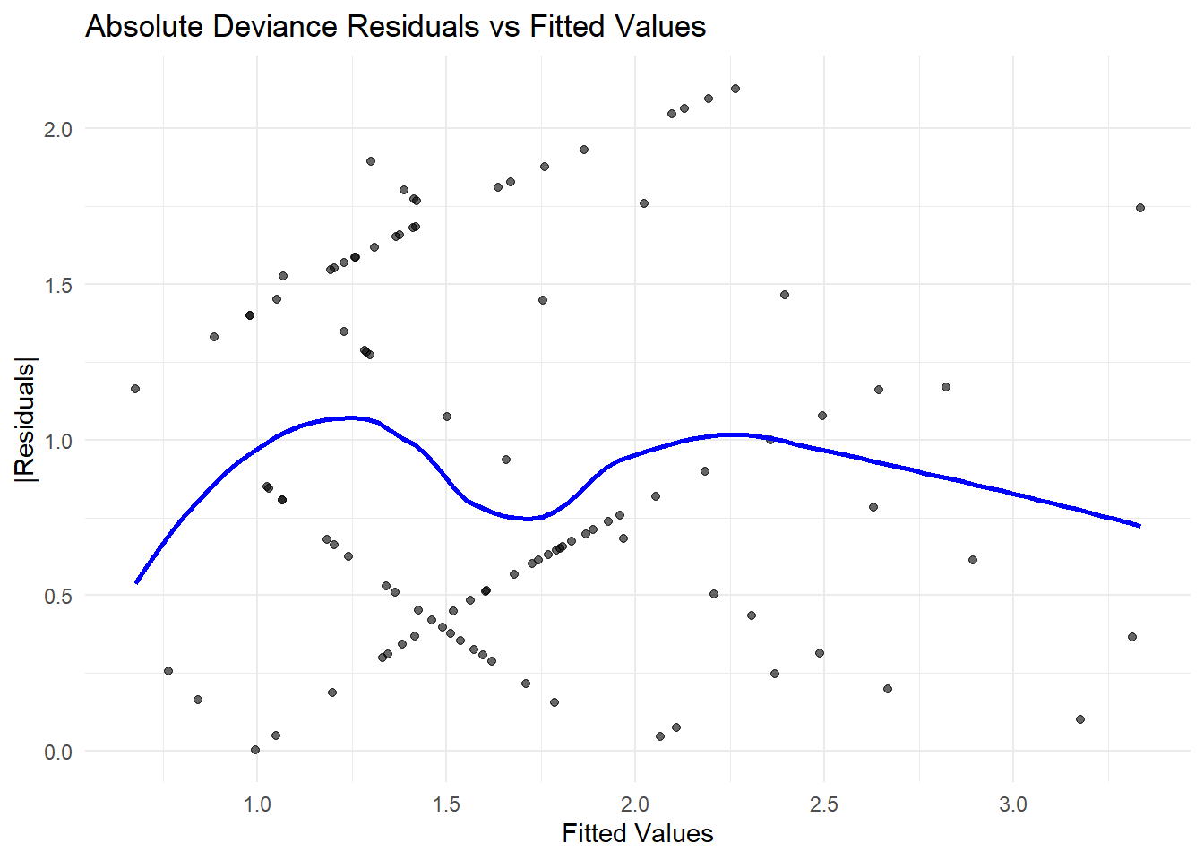
Figure 7.15: Absolute Deviance Residuals vs Fitted Values
# Goodness-of-Fit Metrics
AIC(model_pois)    # Akaike Information Criterion
#> [1] 322.9552
BIC(model_pois)    # Bayesian Information Criterion
#> [1] 328.1655
logLik(model_pois) # Log-likelihood
#> 'log Lik.' -159.4776 (df=2)

# R-squared for GLM
r_squared <-
    1 - (logLik(model_pois) / logLik(glm(y ~ 1, family = poisson)))
r_squared
#> 'log Lik.' 0.05192856 (df=2)

# Overdispersion Check
resid_pearson <- residuals(model_pois, type = "pearson")
# Estimated dispersion parameter
phi_hat <-
    sum(resid_pearson ^ 2) / (n - length(coef(model_pois)))
phi_hat
#> [1] 1.055881

# If phi > 1,
# fit a Negative Binomial Model to correct for overdispersion
if (phi_hat > 1) {
    model_nb <- glm.nb(y ~ x)
    summary(model_nb)
}
#>
#> Call:
#> glm.nb(formula = y ~ x, init.theta = 50.70707605, link = log)
#>
#> Coefficients:
#>             Estimate Std. Error z value Pr(>|z|)
#> (Intercept)  0.42913    0.08514   5.040 4.65e-07 ***
#> x            0.35262    0.08654   4.075 4.61e-05 ***
#> ---
#> Signif. codes:  0 '***' 0.001 '**' 0.01 '*' 0.05 '.' 0.1 ' ' 1
#>
#> (Dispersion parameter for Negative Binomial(50.7071) family taken to be 1)
#>
#>     Null deviance: 135.71  on 99  degrees of freedom
#> Residual deviance: 118.92  on 98  degrees of freedom
#> AIC: 324.91
#>
#> Number of Fisher Scoring iterations: 1
#>
#>
#>               Theta:  51
#>           Std. Err.:  233
#>
#> 2 x log-likelihood: -318.906- Standardized Residuals vs. Fitted Values
If there is a clear trend in the residual plot (e.g., a curve), this suggests an incorrect link function.
If the residual spread increases with fitted values, the variance function may be misspecified.
- Absolute Residuals vs. Fitted Values
A systematic pattern (e.g., funnel shape) suggests heteroscedasticity (i.e., changing variance).
If the residuals increase with fitted values, a different variance function (e.g., Negative Binomial instead of Poisson) may be needed.
- Goodness-of-Fit Metrics
AIC/BIC: Lower values indicate a better model, but must be compared across nested models.
Log-likelihood: Higher values suggest a better-fitting model.
\(R^2\) for GLMs: Since traditional \(R^2\) is not available, the likelihood-based \(R^2\) is used to measure improvement over a null model.
- Overdispersion Check (\(\phi\))
If \(\phi \approx 1\), the Poisson assumption is valid.
If \(\phi > 1\), there is overdispersion, meaning a Negative Binomial model may be more appropriate.
If \(\phi < 1\), underdispersion is present, requiring alternative distributions like the Conway-Maxwell Poisson.