30.3 Simple Difference-in-Differences
DID first emerged as an econometric workhorse for natural experiments, settings where policy shocks or geographic quirks mimic random assignment. Since then, its reach has grown dramatically: marketing A/B roll-outs, corporate ESG mandates, even the staggered release of a mobile-app feature now routinely call on DID for credible impact estimates.
At its computational heart lies the Fixed Effects Estimator, which sweeps out any time-invariant heterogeneity across units and any shocks common to all periods—making DID a cornerstone technique for causal inference in observational data.
DID cleverly harnesses inter-temporal variation between groups in two complementary ways to fight omitted variable bias:
- Cross-sectional comparison: Compares treated and control units at the same point in time, canceling bias from shocks that hit both groups equally (e.g., nationwide inflation). This helps avoid omitted variable bias due to common trends.
- Time-series comparison: Tracks the same unit over time, purging bias from any fixed, unit-specific traits (e.g., a chain’s brand equity, a region’s climate). This helps mitigate omitted variable bias due to cross-sectional heterogeneity.
By taking the difference of differences, we simultaneously:
- Remove common trends that could confound a simple cross-sectional comparison.
- Eliminate unit-specific constants that would spoil a pure time-series analysis.
30.3.1 Basic Setup of DID
Consider a simple setting in Table 30.1 with:
- Treatment Group (\(D_i = 1\))
- Control Group (\(D_i = 0\))
- Pre-Treatment Period (\(T = 0\))
- Post-Treatment Period (\(T = 1\))
| After Treatment (\(T = 1\)) | Before Treatment (\(T = 0\)) | |
|---|---|---|
| Treated (\(D_i = 1\)) | \(E[Y_{1i}(1)|D_i = 1]\) | \(E[Y_{0i}(0)|D_i = 1]\) |
| Control (\(D_i = 0\)) | \(E[Y_{0i}(1)|D_i = 0]\) | \(E[Y_{0i}(0)|D_i = 0]\) |
The fundamental challenge: We cannot observe \(E[Y_{0i}(1)|D_i = 1]\) (i.e., the counterfactual outcome for the treated group had they not received treatment).
DID estimates the Average Treatment Effect on the Treated using the following formula:
\[ \begin{aligned} E[Y_1(1) - Y_0(1) | D = 1] &= \{E[Y(1)|D = 1] - E[Y(1)|D = 0] \} \\ &- \{E[Y(0)|D = 1] - E[Y(0)|D = 0] \} \end{aligned} \]
This formulation differences out time-invariant unobserved factors, assuming the parallel trends assumption holds.
- For the treated group, we isolate the difference between being treated and not being treated.
- If the control group would have experienced a different trajectory, the DID estimate may be biased.
- Since we cannot observe treatment variation in the control group, we cannot infer the treatment effect for this group.
# Load required libraries
library(dplyr)
library(ggplot2)
set.seed(1)

# Simulated dataset for illustration
data <- data.frame(
  time = rep(c(0, 1), each = 50),  # Pre (0) and Post (1)
  treated = rep(c(0, 1), times = 50), # Control (0) and Treated (1)
  error = rnorm(100)
)

# Generate outcome variable
data$outcome <-
    5 + 3 * data$treated + 2 * data$time +
    4 * data$treated * data$time + data$error

# Compute averages for 2x2 table
table_means <- data %>%
  group_by(treated, time) %>%
  summarize(mean_outcome = mean(outcome), .groups = "drop") %>%
  mutate(
    group = paste0(ifelse(treated == 1, "Treated", "Control"), ", ",
                   ifelse(time == 1, "Post", "Pre"))
  )

# Display the 2x2 table
table_2x2 <- table_means %>%
  select(group, mean_outcome) %>%
  tidyr::spread(key = group, value = mean_outcome)

print("2x2 Table of Mean Outcomes:")
#> [1] "2x2 Table of Mean Outcomes:"
print(table_2x2)
#> # A tibble: 1 × 4
#>   `Control, Post` `Control, Pre` `Treated, Post` `Treated, Pre`
#>             <dbl>          <dbl>           <dbl>          <dbl>
#> 1            7.19           5.20            14.0           8.00

# Calculate Diff-in-Diff manually

# Treated, Post
Y11 <- table_means$mean_outcome[table_means$group == "Treated, Post"]

# Treated, Pre
Y10 <- table_means$mean_outcome[table_means$group == "Treated, Pre"]

# Control, Post
Y01 <- table_means$mean_outcome[table_means$group == "Control, Post"]

# Control, Pre
Y00 <- table_means$mean_outcome[table_means$group == "Control, Pre"]

diff_in_diff_formula <- (Y11 - Y10) - (Y01 - Y00)

# Estimate DID using OLS
model <- lm(outcome ~ treated * time, data = data)
ols_estimate <- coef(model)["treated:time"]

# Print results
results <- data.frame(
  Method = c("Diff-in-Diff Formula", "OLS Estimate"),
  Estimate = c(diff_in_diff_formula, ols_estimate)
)

print("Comparison of DID Estimates:")
#> [1] "Comparison of DID Estimates:"
print(results)
#>                            Method Estimate
#>              Diff-in-Diff Formula 4.035895
#> treated:time         OLS Estimate 4.035895
Figure 30.5 shows a simple visualization of the DID in practice.
# Visualization
ggplot(data,
       aes(
           x = as.factor(time),
           y = outcome,
           color = as.factor(treated),
           group = treated
       )) +
    stat_summary(fun = mean, geom = "point", size = 3) +
    stat_summary(fun = mean,
                 geom = "line",
                 linetype = "dashed") +
    labs(
        title = "Difference-in-Differences Visualization",
        x = "Time (0 = Pre, 1 = Post)",
        y = "Outcome",
        color = "Group"
    ) +
    scale_color_manual(labels = c("Control", "Treated"),
                       values = c("blue", "red")) +
    causalverse::ama_theme()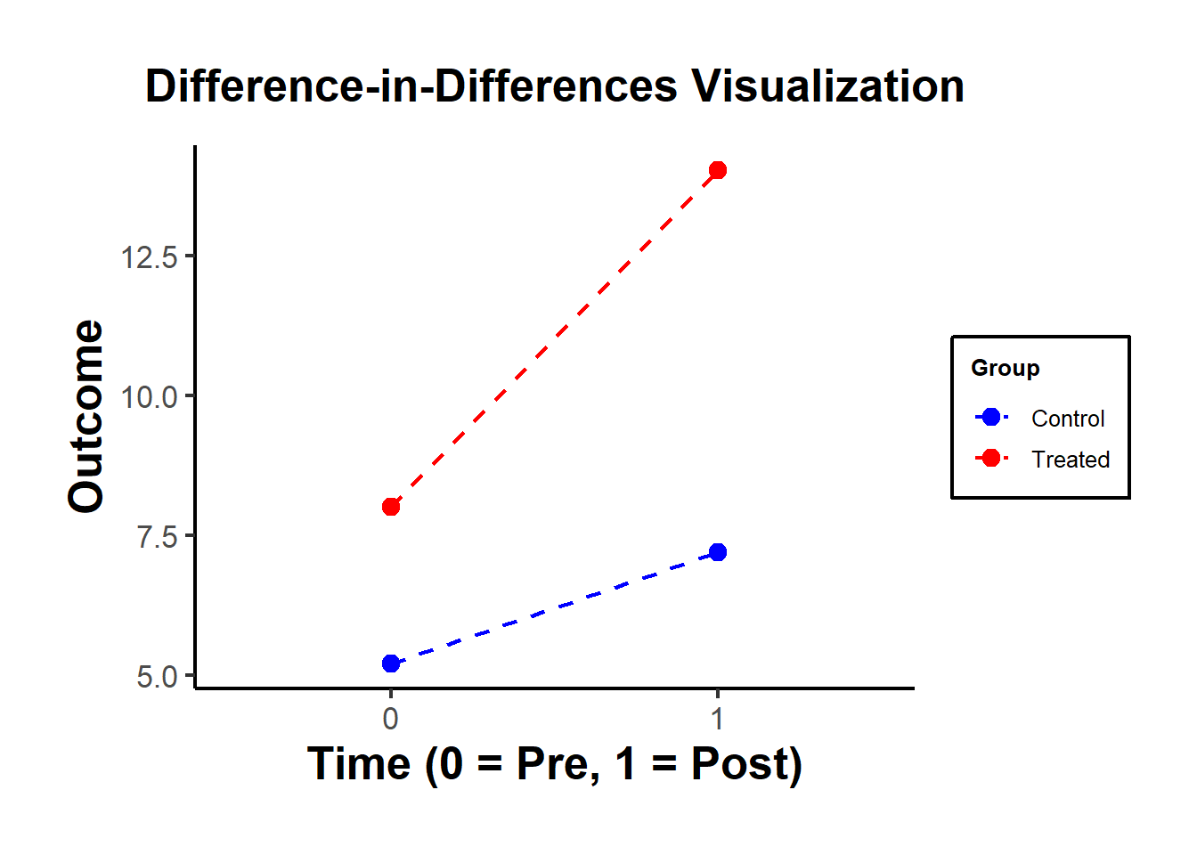
Figure 30.5: DiD Visualization
| Control (0) | Treated (1) | |
|---|---|---|
| Pre (0) | \(\bar{Y}_{00} = 5\) | \(\bar{Y}_{10} = 8\) |
| Post (1) | \(\bar{Y}_{01} = 7\) | \(\bar{Y}_{11} = 14\) |
Table 30.2 organizes the mean outcomes into four cells:
Control Group, Pre-period (\(\bar{Y}_{00}\)): Mean outcome for the control group before the intervention.
Control Group, Post-period (\(\bar{Y}_{01}\)): Mean outcome for the control group after the intervention.
Treated Group, Pre-period (\(\bar{Y}_{10}\)): Mean outcome for the treated group before the intervention.
Treated Group, Post-period (\(\bar{Y}_{11}\)): Mean outcome for the treated group after the intervention.
The DID treatment effect calculated from the simple formula of averages is identical to the estimate from an OLS regression with an interaction term.
The treatment effect is calculated as:
\(\text{DID} = (\bar{Y}_{11} - \bar{Y}_{10}) - (\bar{Y}_{01} - \bar{Y}_{00})\)
Compute manually:
\((\bar{Y}_{11} - \bar{Y}_{10}) - (\bar{Y}_{01} - \bar{Y}_{00})\)
Use OLS regression:
\(Y_{it} = \beta_0 + \beta_1 \text{treated}_i + \beta_2 \text{time}_t + \beta_3 (\text{treated}_i \cdot \text{time}_t) + \epsilon_{it}\)
Using the simulated table:
\(\text{DID} = (14 - 8) - (7 - 5) = 6 - 2 = 4\)
This matches the interaction term coefficient (\(\beta_3 = 4\)) from the OLS regression.
Both methods give the same result!
30.3.2 Extensions of DID
30.3.2.1 DID with More Than Two Groups or Time Periods
DID can be extended to multiple treatments, multiple controls, and more than two periods:
\[ Y_{igt} = \alpha_g + \gamma_t + \beta I_{gt} + \delta X_{igt} + \epsilon_{igt} \]
where:
\(\alpha_g\) = Group-Specific Fixed Effects (e.g., firm, region).
\(\gamma_t\) = Time-Specific Fixed Effects (e.g., year, quarter).
\(\beta\) = DID Effect.
\(I_{gt}\) = Interaction Terms (Treatment × Post-Treatment).
\(\delta X_{igt}\) = Additional Covariates.
This is known as the Two-Way Fixed Effects DID model. However, TWFE performs poorly under staggered treatment adoption, where different groups receive treatment at different times.
30.3.2.2 Examining Long-Term Effects (Dynamic DID)
To examine the dynamic treatment effects (that are not under rollout/staggered design), we can create a centered time variable (Table 30.3).
| Centered Time Variable | Interpretation |
|---|---|
| \(t = -2\) | Two periods before treatment |
| \(t = -1\) | One period before treatment |
| \(t = 0\) | Last pre-treatment period right before treatment period (Baseline/Reference Group) |
| \(t = 1\) | Treatment period |
| \(t = 2\) | One period after treatment |
Dynamic Treatment Model Specification
By interacting this factor variable, we can examine the dynamic effect of treatment (i.e., whether it’s fading or intensifying):
\[ \begin{aligned} Y &= \alpha_0 + \alpha_1 Group + \alpha_2 Time \\ &+ \beta_{-T_1} Treatment + \beta_{-(T_1 -1)} Treatment + \dots + \beta_{-1} Treatment \\ &+ \beta_1 + \dots + \beta_{T_2} Treatment \end{aligned} \]
where:
\(\beta_0\) (Baseline Period) is the reference group (i.e., drop from the model).
\(T_1\) = Pre-Treatment Period.
\(T_2\) = Post-Treatment Period.
Treatment coefficients (\(\beta_t\)) measure the effect over time.
Key Observations:
Pre-treatment coefficients should be close to zero (\(\beta_{-T_1}, \dots, \beta_{-1} \approx 0\)), ensuring no pre-trend bias.
Post-treatment coefficients should be significantly different from zero (\(\beta_1, \dots, \beta_{T_2} \neq 0\)), measuring the treatment effect over time.
Higher standard errors with more interactions: Including too many lags can reduce precision.
30.3.2.3 DID on Relationships, Not Just Levels
While DID is most commonly applied to examine treatment effects on outcome levels, it can also be used to estimate how treatment affects the relationship between variables. This approach treats estimated coefficients from first-stage regressions as outcomes in a second-stage DID analysis.
Standard DID examines whether treatment changes the level of an outcome \(Y_{it}\). However, researchers may be interested in whether treatment changes how \(Y\) responds to some predictor \(X\), that is, whether treatment affects the coefficient \(\beta\) in the relationship:
\[ Y_{it} = \alpha + \beta X_{it} + \epsilon_{it} \]
This requires a two-stage approach where regression coefficients themselves become the unit of analysis.
Two-Stage Estimation Procedure
Stage 1: Estimate Group-Period-Specific Relationships
For each combination of group \(g\) and time period \(t\), estimate:
\[ Y_{igt} = \alpha_{gt} + \beta_{gt} X_{igt} + \epsilon_{igt} \]
This yields a set of estimated coefficients \(\{\hat{\beta}_{gt}\}\), where each \(\hat{\beta}_{gt}\) captures the relationship between \(X\) and \(Y\) for group \(g\) in period \(t\).
Stage 2: Apply DID to the Estimated Coefficients
Treat the estimated coefficients \(\hat{\beta}_{gt}\) as the outcome variable in a standard DID framework:
\[ \hat{\beta}_{gt} = \alpha_0 + \alpha_1 Treated_g + \alpha_2 Post_t + \delta (Treated_g \times Post_t) + u_{gt} \]
where:
- \(\hat{\beta}_{gt}\) = Estimated coefficient from Stage 1 (the “outcome”).
- \(Treated_g\) = Indicator for treatment group.
- \(Post_t\) = Indicator for post-treatment period.
- \(\delta\) = DID estimate of treatment effect on the relationship.
The coefficient \(\delta\) measures whether the relationship between \(X\) and \(Y\) changed differentially for the treated group after treatment.
The DID estimator can be expressed as:
\[ \begin{aligned} \hat{\delta} &= (\hat{\beta}_{Treated}^{Post} - \hat{\beta}_{Treated}^{Pre}) - (\hat{\beta}_{Control}^{Post} - \hat{\beta}_{Control}^{Pre}) \\ &= \text{Change in relationship for treated} - \text{Change in relationship for control} \end{aligned} \]
This captures the causal effect of treatment on the structural parameter \(\beta\), controlling for secular trends that affect both groups.
30.3.2.3.1 Example: Price Sensitivity Before and After a Policy Change
Suppose we want to test whether a consumer protection law changes how price affects demand.
Stage 1: For each state \(s\) and year \(t\), estimate:
\[ \log(Quantity_{ist}) = \alpha_{st} + \beta_{st} \log(Price_{ist}) + \epsilon_{ist} \]
where \(i\) indexes individual transactions. This gives us state-year specific price elasticities \(\{\hat{\beta}_{st}\}\).
Stage 2: Use these elasticities as outcomes in a DID model:
\[ \hat{\beta}_{st} = \alpha_0 + \alpha_1 Treated_s + \alpha_2 Post_t + \delta (Treated_s \times Post_t) + u_{st} \]
If \(\delta < 0\), the policy made consumers more price-sensitive (more elastic demand) in treated states. If \(\delta > 0\), consumers became less price-sensitive.
30.3.2.3.2 Standard Error Correction
A critical issue is that Stage 2 uses estimated coefficients \(\hat{\beta}_{gt}\) as the dependent variable, which introduces generated regressor problems. The standard errors from Stage 2 are incorrect because they don’t account for estimation uncertainty in \(\hat{\beta}_{gt}\).
Solutions:
Bootstrapping: Resample at the individual level, re-estimate both stages, and calculate standard errors from the bootstrap distribution.
Weighted Least Squares: Weight Stage 2 observations by the inverse of the variance of \(\hat{\beta}_{gt}\):
\[ w_{gt} = \frac{1}{\text{Var}(\hat{\beta}_{gt})} = \frac{1}{SE(\hat{\beta}_{gt})^2} \]
This gives more weight to precisely estimated relationships.
- Stacked Regression: Pool all individual observations and include group-period fixed effects interacted with \(X\):
\[ Y_{igt} = \sum_{g,t} \beta_{gt} (I_{gt} \times X_{igt}) + \text{controls} + \epsilon_{igt} \]
Then test whether \(\{\beta_{gt}\}\) follow a DID pattern using an F-test or linear combinations.
30.3.2.3.3 Dynamic Effects on Relationships
The two-stage approach can be extended to examine how relationships evolve over time:
Stage 1: Estimate period-specific coefficients:
\[ Y_{igt} = \alpha_{gt} + \beta_{gt} X_{igt} + \epsilon_{igt} \]
Stage 2: Event study specification:
\[ \hat{\beta}_{gt} = \alpha_g + \gamma_t + \sum_{k \neq -1} \delta_k (Treated_g \times Period_{t=k}) + u_{gt} \]
where \(Period_{t=k}\) are indicators for time relative to treatment (with \(k=-1\) as the reference period).
Key Observations:
- Pre-treatment coefficients (\(\delta_k\) for \(k < -1\)) should be near zero, indicating parallel trends in the relationship.
- Post-treatment coefficients (\(\delta_k\) for \(k \geq 0\)) show how the relationship evolves after treatment.
- This reveals whether effects on relationships are immediate, delayed, or fade over time.
30.3.2.3.4 Applications
1. Advertising Effectiveness:
Does a competitor’s market entry change advertising elasticity?
- Stage 1: Estimate \(\frac{\partial \log(Sales)}{\partial \log(Advertising)}\) for each market-period.
- Stage 2: DID on these elasticities comparing markets with/without competitor entry.
2. Labor Supply Elasticity:
Does a tax reform change labor supply responsiveness to wages?
- Stage 1: Estimate \(\frac{\partial Hours}{\partial Wage}\) for each region-year.
- Stage 2: DID comparing regions with different tax policy changes.
3. Educational Returns:
Does a curriculum reform change the returns to study time?
- Stage 1: Estimate \(\frac{\partial GPA}{\partial StudyHours}\) for each school-year.
- Stage 2: DID comparing schools that adopted vs. didn’t adopt the reform.
4. Platform Network Effects:
Does a platform algorithm change affect network externalities?
- Stage 1: Estimate \(\frac{\partial UserValue}{\partial NetworkSize}\) for each market-quarter.
- Stage 2: DID around the algorithm change.
30.3.2.3.5 Advantages and Limitations
Advantages:
- Causal inference on mechanisms: Identifies how treatment changes behavioral responses, not just outcomes.
- Flexibility: Can be applied to any estimable relationship (elasticities, marginal effects, coefficients).
- Policy-relevant: Directly tests whether policies alter structural parameters of interest.
Limitations:
- Two-stage uncertainty: Standard errors require careful correction for generated regressors.
- Data requirements: Needs sufficient observations within each group-period to estimate first-stage relationships precisely.
- Parallel trends in relationships: Requires that relationships (not just levels) would have trended similarly absent treatment—a stronger assumption.
- Aggregation: Loses individual-level variation when collapsing to group-period coefficients.
30.3.2.3.6 Relationship to Heterogeneous Treatment Effects
DID on relationships is conceptually related to, but distinct from, heterogeneous treatment effects. A three-way interaction \((X \times Treated \times Post)\) estimates whether treatment effects vary across levels of \(X\). In contrast, DID on relationships estimates whether the effect of \(X\) on \(Y\) changes due to treatment, a fundamentally different question about structural parameters rather than treatment heterogeneity.
This two-stage approach transforms DID into a tool for testing structural change hypotheses, enabling researchers to make causal claims about how treatments alter the fundamental relationships governing economic, social, or behavioral systems.
30.3.3 Goals of DID
- Pre-Treatment Coefficients Should Be Insignificant
- Ensure that \(\beta_{-T_1}, \dots, \beta_{-1} = 0\) (similar to a Placebo Test).
- Post-Treatment Coefficients Should Be Significant
- Verify that \(\beta_1, \dots, \beta_{T_2} \neq 0\).
- Examine whether the trend in post-treatment coefficients is increasing or decreasing over time.
library(tidyverse)
library(fixest)

od <- causaldata::organ_donations %>%

    # Treatment variable
    dplyr::mutate(California = State == 'California') %>%
    # centered time variable
    dplyr::mutate(center_time = as.factor(Quarter_Num - 3))
# where 3 is the reference period precedes the treatment period

class(od$California)
#> [1] "logical"
class(od$State)
#> [1] "character"

cali <- feols(Rate ~ i(center_time, California, ref = 0) |
                  State + center_time,
              data = od)

etable(cali)
#>                                           cali
#> Dependent Var.:                           Rate
#>
#> California x center_time = -2 -0.0029 (0.0360)
#> California x center_time = -1  0.0063 (0.0360)
#> California x center_time = 1  -0.0216 (0.0360)
#> California x center_time = 2  -0.0203 (0.0360)
#> California x center_time = 3  -0.0222 (0.0360)
#> Fixed-Effects:                ----------------
#> State                                      Yes
#> center_time                                Yes
#> _____________________________ ________________
#> S.E. type                                  IID
#> Observations                               162
#> R2                                     0.97934
#> Within R2                              0.00979
#> ---
#> Signif. codes: 0 '***' 0.001 '**' 0.01 '*' 0.05 '.' 0.1 ' ' 1
Figure 30.6 shows the fixed effects estimates over time.
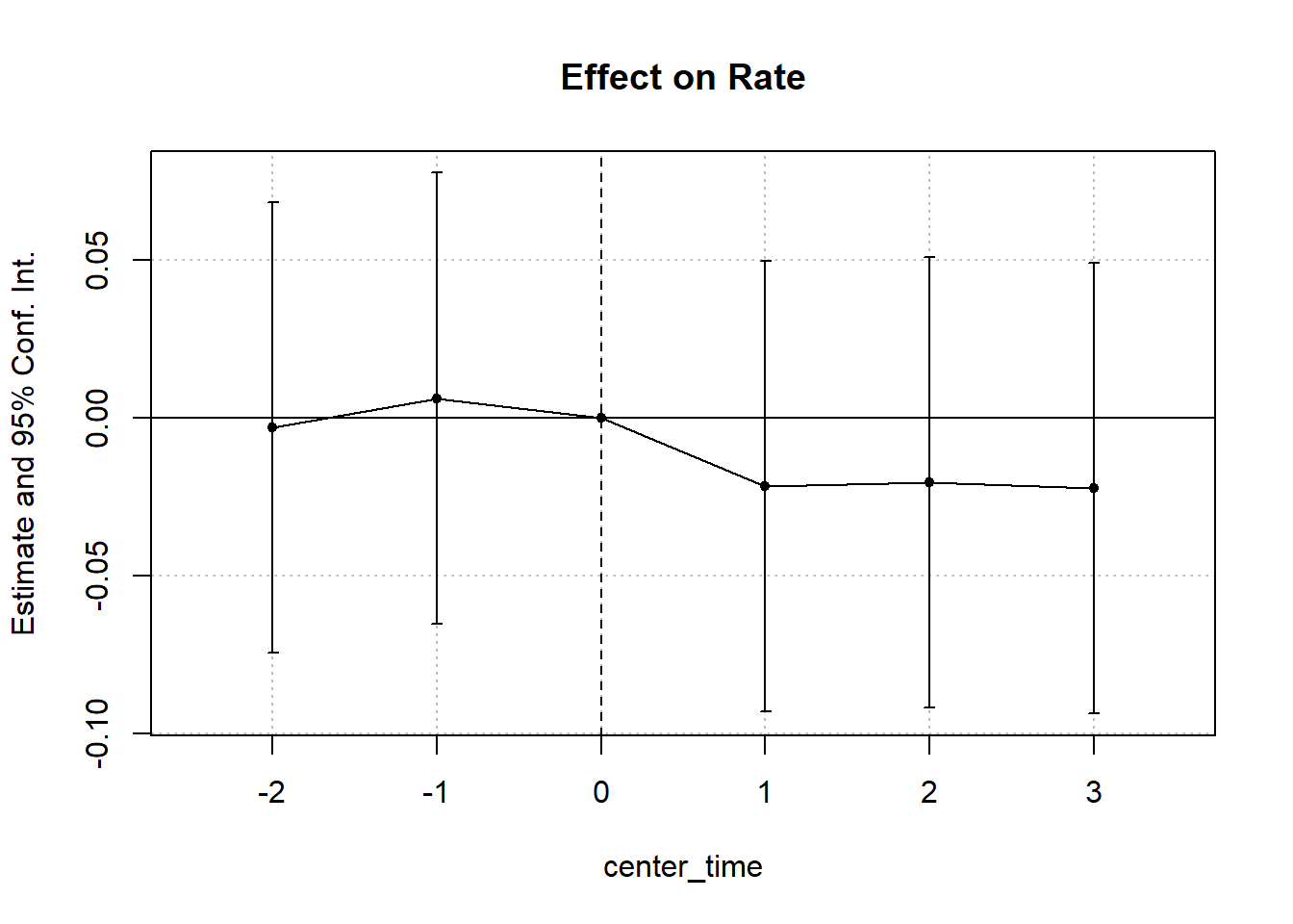
Figure 30.6: Estimated Effect on Rate Over Time
Figure 30.7 shows the same plot with a different plotting function.
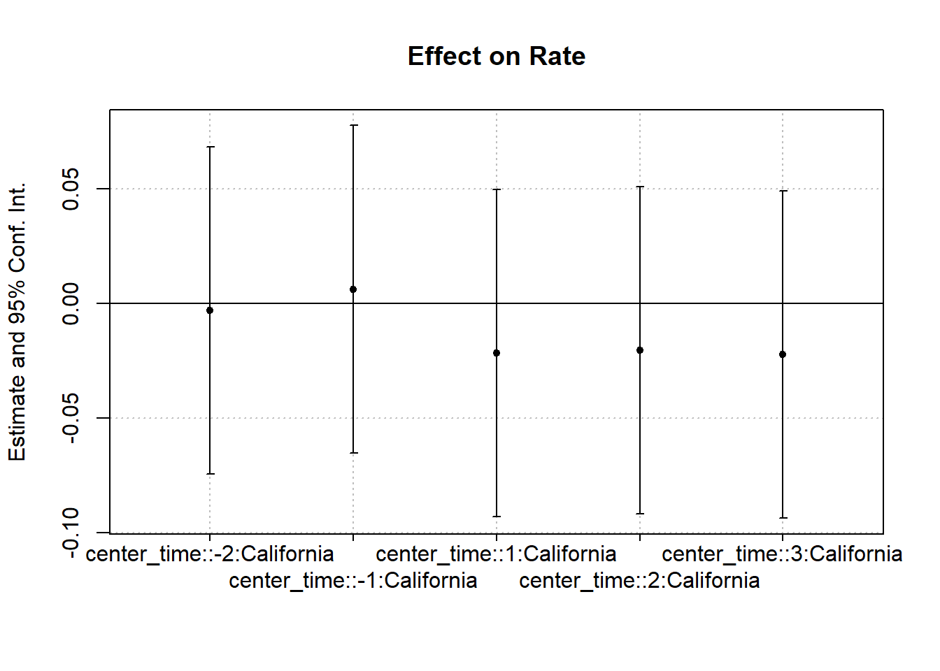
Figure 30.7: Interaction Effect on Rate