8.5 Split-Plot Designs
Split-plot designs are commonly used in experimental settings where there are two or more factors, and at least one of them requires larger experimental units compared to the other(s). This situation often arises in agricultural, industrial, and business experiments where certain treatments are harder or more expensive to apply.
Key Characteristics
- Two factors with different experimental unit requirements:
- Factor A (Whole-plot factor): Requires large experimental units (e.g., different fields, production batches).
- Factor B (Sub-plot factor): Can be applied to smaller units within the larger experimental units (e.g., plots within fields, products within batches).
- Blocking: The experiment is typically divided into blocks (or replicates) to account for variability. However, unlike Randomized Block Designs, the randomization process in split-plot designs occurs at two levels:
- Whole-plot randomization: Factor A is randomized across large units within each block.
- Sub-plot randomization: Factor B is randomized within each whole plot.
8.5.1 Example Setup
- Factor A: 3 levels (applied to large units).
- Factor B: 2 levels (applied within the large units).
- 4 Blocks (replicates): Each containing all combinations of A and B.
Unlike in Randomized Block Designs, the randomization of Factor A is restricted due to the larger unit size. Factor A is applied once per block, while Factor B can be applied multiple times within each block.
8.5.2 Statistical Model for Split-Plot Designs
- When Factor A is the Primary Focus (Whole-Plot Analysis)
\[ Y_{ij} = \mu + \rho_i + \alpha_j + e_{ij} \]
Where:
\(Y_{ij}\) = Response for the \(j\)-th level of factor A in the \(i\)-th block.
\(\mu\) = Overall mean.
\(\rho_i\) = Random effect of the \(i\)-th block (\(\rho_i \sim N(0, \sigma^2_{\rho})\)).
\(\alpha_j\) = Fixed effect of factor A (main effect).
\(e_{ij} \sim N(0, \sigma^2_{e})\) = Whole-plot error (random), representing the variability within blocks due to factor A.
- When Factor B is the Primary Focus (Sub-Plot Analysis)
\[ Y_{ijk} = \mu + \phi_{ij} + \beta_k + \epsilon_{ijk} \]
Where:
\(Y_{ijk}\) = Response for the \(k\)-th level of factor B within the \(j\)-th level of factor A and \(i\)-th block.
\(\phi_{ij}\) = Combined effect of block and factor A: \[ \phi_{ij} = \rho_i + \alpha_j + e_{ij} \]
\(\beta_k\) = Fixed effect of factor B (main effect).
\(\epsilon_{ijk} \sim N(0, \sigma^2_{\epsilon})\) = Sub-plot error (random), capturing variability within whole plots.
- Full Split-Plot Model (Including Interaction)
\[ Y_{ijk} = \mu + \rho_i + \alpha_j + e_{ij} + \beta_k + (\alpha \beta)_{jk} + \epsilon_{ijk} \]
Where:
\(i\) = Block (replication). - \(j\) = Level of factor A (whole-plot factor).
\(k\) = Level of factor B (sub-plot factor).
\(\mu\) = Overall mean.
\(\rho_i\) = Random effect of the \(i\)-th block.
\(\alpha_j\) = Fixed main effect of factor A.
\(e_{ij} \sim N(0, \sigma^2_{e})\) = Whole-plot error (random).
\(\beta_k\) = Fixed main effect of factor B.
\((\alpha \beta)_{jk}\) = Fixed interaction effect between factors A and B.
\(\epsilon_{ijk} \sim N(0, \sigma^2_{\epsilon})\) = Sub-plot error (random).
8.5.3 Approaches to Analyzing Split-Plot Designs
- ANOVA Perspective
Whole-Plot Comparisons:
- Factor A vs. Whole-Plot Error:
Compare the variation due to factor A (\(\alpha_j\)) against the whole-plot error (\(e_{ij}\)). - Blocks vs. Whole-Plot Error:
Compare the variation due to blocks (\(\rho_i\)) against the whole-plot error (\(e_{ij}\)).
Sub-Plot Comparisons:
- Factor B vs. Sub-Plot Error:
Compare the variation due to factor B (\(\beta_k\)) against the sub-plot error (\(\epsilon_{ijk}\)). - Interaction (A × B) vs. Sub-Plot Error:
Compare the interaction effect (\((\alpha \beta)_{jk}\)) against the sub-plot error (\(\epsilon_{ijk}\)).
- Mixed Model Perspective
A more flexible approach is to treat split-plot designs using mixed-effects models, which can handle both fixed and random effects explicitly:
\[ \mathbf{Y = X \beta + Zb + \epsilon} \]
Where:
\(\mathbf{Y}\) = Vector of observed responses.
\(\mathbf{X}\) = Design matrix for fixed effects (e.g., factors A, B, and their interaction).
\(\boldsymbol{\beta}\) = Vector of fixed-effect coefficients (e.g., \(\mu\), \(\alpha_j\), \(\beta_k\), \((\alpha \beta)_{jk}\)).
\(\mathbf{Z}\) = Design matrix for random effects (e.g., blocks and whole-plot errors).
\(\mathbf{b}\) = Vector of random-effect coefficients (e.g., \(\rho_i\), \(e_{ij}\)).
\(\boldsymbol{\epsilon}\) = Vector of residuals (sub-plot error).
Mixed models are particularly useful when:
There are unbalanced designs (missing data).
You need to account for complex correlation structures within the data.
8.5.4 Application: Split-Plot Design
Consider an agricultural experiment designed to study the effects of irrigation and crop variety on yield. This scenario is well-suited for a split-plot design because irrigation treatments are applied to large plots (fields), while different crop varieties are planted within these plots.
8.5.4.1 Model Specification
The linear mixed-effects model is defined as:
\[ y_{ijk} = \mu + i_i + v_j + (iv)_{ij} + f_k + \epsilon_{ijk} \]
Where:
\(y_{ijk}\) = Observed yield for the \(i\)-th irrigation, \(j\)-th variety, in the \(k\)-th field.
\(\mu\) = Overall mean yield.
\(i_i\) = Fixed effect of the \(i\)-th irrigation level.
\(v_j\) = Fixed effect of the \(j\)-th crop variety.
\((iv)_{ij}\) = Interaction effect between irrigation and variety (fixed).
\(f_k \sim N(0, \sigma^2_f)\) = Random effect of field (captures variability between fields).
\(\epsilon_{ijk} \sim N(0, \sigma^2_\epsilon)\) = Residual error.
Note:
Since each variety-field combination is observed only once, we cannot model a random interaction between variety and field.
8.5.4.2 Data Exploration
library(ggplot2)
data(irrigation, package = "faraway")  # Load the dataset

# Summary statistics and preview
summary(irrigation)
#>      field   irrigation variety     yield
#>  f1     :2   i1:4       v1:8    Min.   :34.80
#>  f2     :2   i2:4       v2:8    1st Qu.:37.60
#>  f3     :2   i3:4               Median :40.15
#>  f4     :2   i4:4               Mean   :40.23
#>  f5     :2                      3rd Qu.:42.73
#>  f6     :2                      Max.   :47.60
#>  (Other):4
head(irrigation, 4)
#>   field irrigation variety yield
#> 1    f1         i1      v1  35.4
#> 2    f1         i1      v2  37.9
#> 3    f2         i2      v1  36.7
#> 4    f2         i2      v2  38.2
# Exploratory plot
ggplot(irrigation,
aes(
x = field,
y = yield,
shape = irrigation,
color = variety
)) +
geom_point(size = 3) +
labs(title = "Yield by Field, Irrigation, and Variety",
x = "Field",
y = "Yield") +
theme_minimal()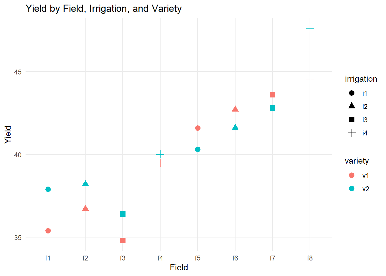
Figure 8.1: Yield by Field, Irrigation, and Variety
This plot helps visualize how yield varies across fields, under different irrigation treatments, and for different varieties.
8.5.4.3 Fitting the Initial Mixed-Effects Model
We fit a mixed-effects model where:
Irrigation and variety (and their interaction) are fixed effects.
Field is modeled as a random effect to account for variability between fields.
library(lmerTest)  # Provides p-values for lmer models

# Full model with interaction term
sp_model <-
  lmer(yield ~ irrigation * variety
       + (1 | field), data = irrigation)
summary(sp_model)
#> Linear mixed model fit by REML. t-tests use Satterthwaite's method [
#> lmerModLmerTest]
#> Formula: yield ~ irrigation * variety + (1 | field)
#>    Data: irrigation
#>
#> REML criterion at convergence: 45.4
#>
#> Scaled residuals:
#>     Min      1Q  Median      3Q     Max
#> -0.7448 -0.5509  0.0000  0.5509  0.7448
#>
#> Random effects:
#>  Groups   Name        Variance Std.Dev.
#>  field    (Intercept) 16.200   4.025
#>  Residual              2.107   1.452
#> Number of obs: 16, groups:  field, 8
#>
#> Fixed effects:
#>                        Estimate Std. Error     df t value Pr(>|t|)
#> (Intercept)              38.500      3.026  4.487  12.725 0.000109 ***
#> irrigationi2              1.200      4.279  4.487   0.280 0.791591
#> irrigationi3              0.700      4.279  4.487   0.164 0.877156
#> irrigationi4              3.500      4.279  4.487   0.818 0.454584
#> varietyv2                 0.600      1.452  4.000   0.413 0.700582
#> irrigationi2:varietyv2   -0.400      2.053  4.000  -0.195 0.855020
#> irrigationi3:varietyv2   -0.200      2.053  4.000  -0.097 0.927082
#> irrigationi4:varietyv2    1.200      2.053  4.000   0.584 0.590265
#> ---
#> Signif. codes:  0 '***' 0.001 '**' 0.01 '*' 0.05 '.' 0.1 ' ' 1
#>
#> Correlation of Fixed Effects:
#>             (Intr) irrgt2 irrgt3 irrgt4 vrtyv2 irr2:2 irr3:2
#> irrigation2 -0.707
#> irrigation3 -0.707  0.500
#> irrigation4 -0.707  0.500  0.500
#> varietyv2   -0.240  0.170  0.170  0.170
#> irrgtn2:vr2  0.170 -0.240 -0.120 -0.120 -0.707
#> irrgtn3:vr2  0.170 -0.120 -0.240 -0.120 -0.707  0.500
#> irrgtn4:vr2  0.170 -0.120 -0.120 -0.240 -0.707  0.500  0.500

# ANOVA table using Kenward-Roger approximation for accurate p-values
anova(sp_model, ddf = "Kenward-Roger")
#> Type III Analysis of Variance Table with Kenward-Roger's method
#>                    Sum Sq Mean Sq NumDF DenDF F value Pr(>F)
#> irrigation         2.4545 0.81818     3     4  0.3882 0.7685
#> variety            2.2500 2.25000     1     4  1.0676 0.3599
#> irrigation:variety 1.5500 0.51667     3     4  0.2452 0.8612
Check the p-value of the interaction term (
irrigation:variety).- If insignificant, this suggests no strong evidence of an interaction effect, and we may simplify the model by removing it.
8.5.4.4 Model Simplification: Testing for Additivity
We compare the full model (with interaction) to an additive model (without interaction):
library(lme4)

# Additive model (no interaction)
sp_model_additive <- lmer(yield ~ irrigation + variety + (1 | field), data = irrigation)

# Likelihood ratio test comparing the two models
anova(sp_model_additive, sp_model, ddf = "Kenward-Roger")
#> Data: irrigation
#> Models:
#> sp_model_additive: yield ~ irrigation + variety + (1 | field)
#> sp_model: yield ~ irrigation * variety + (1 | field)
#>                   npar    AIC    BIC  logLik -2*log(L)  Chisq Df Pr(>Chisq)
#> sp_model_additive    7 83.959 89.368 -34.980    69.959
#> sp_model            10 88.609 96.335 -34.305    68.609 1.3503  3     0.7172
Hypotheses:
\(H_0\): The additive model (without interaction) fits the data adequately.
\(H_a\): The interaction model provides a significantly better fit.
Interpretation:
If the p-value is insignificant, we fail to reject \(H_0\), meaning the simpler additive model is sufficient.
Check AIC and BIC: Lower values indicate a better-fitting model, supporting the use of the additive model if consistent with the hypothesis test.
8.5.4.5 Assessing the Random Effect: Exact Restricted Likelihood Ratio Test
To verify whether the random field effect is necessary, we conduct an exact RLRT:
Hypotheses:
\(H_0\): \(\sigma^2_f = 0\) (no variability between fields; random effect is unnecessary).
\(H_a\): \(\sigma^2_f > 0\) (random field effect is significant).
library(RLRsim)

# RLRT for the random effect of field
exactRLRT(sp_model)
#>
#>  simulated finite sample distribution of RLRT.
#>
#>  (p-value based on 10000 simulated values)
#>
#> data:
#> RLRT = 6.1118, p-value = 0.01
Interpretation:
If the p-value is significant, we reject \(H_0\), confirming that the random field effect is essential.
A significant random effect implies substantial variability between fields that must be accounted for in the model.