10.8 Regression Trees and Random Forests
Though not typically framed as “kernel” or “spline,” tree-based methods—such as Classification and Regression Trees (CART) and random forests—are also nonparametric models. They do not assume a predetermined functional form for the relationship between predictors and the response. Instead, they adaptively partition the predictor space into regions, fitting simple models (usually constants or linear models) within each region.
10.8.1 Regression Trees
The Classification and Regression Trees (CART) algorithm is the foundation of tree-based models (Breiman 2017). In regression settings, CART models the response variable as a piecewise constant function.
A regression tree recursively partitions the predictor space into disjoint regions, \(R_1, R_2, \ldots, R_M\), and predicts the response as a constant within each region:
\[ \hat{m}(x) = \sum_{m=1}^{M} c_m \cdot \mathbb{I}(x \in R_m), \]
where:
- \(c_m\) is the predicted value (usually the mean of \(y_i\)) for all observations in region \(R_m\),
- \(\mathbb{I}(\cdot)\) is the indicator function.
Tree-Building Algorithm (Greedy Recursive Partitioning):
- Start with the full dataset as a single region.
- Find the best split:
- Consider all possible splits of all predictors (e.g., \(X_j < s\)).
- Choose the split that minimizes the residual sum of squares (RSS): \[ \text{RSS} = \sum_{i \in R_1} (y_i - \bar{y}_{R_1})^2 + \sum_{i \in R_2} (y_i - \bar{y}_{R_2})^2, \] where \(\bar{y}_{R_k}\) is the mean response in region \(R_k\).
- Recursively repeat the splitting process for each new region (node) until a stopping criterion is met (e.g., minimum number of observations per leaf, maximum tree depth).
- Assign a constant prediction to each terminal node (leaf) based on the average response of observations within that node.
Stopping Criteria and Pruning:
- Pre-pruning (early stopping): Halt the tree growth when a predefined condition is met (e.g., minimal node size, maximal depth).
- Post-pruning (cost-complexity pruning): Grow a large tree first, then prune back to avoid overfitting. The cost-complexity criterion is: \[ C_\alpha(T) = \text{RSS}(T) + \alpha |T|, \] where \(|T|\) is the number of terminal nodes (leaves) and \(\alpha\) controls the penalty for complexity.
Advantages of Regression Trees:
- Interpretability: Easy to visualize and understand.
- Handling of different data types: Can naturally handle numerical and categorical variables.
- Nonlinear relationships and interactions: Captures complex patterns without explicit modeling.
Limitations:
- High variance: Trees are sensitive to small changes in data (unstable).
- Overfitting risk: Without pruning or regularization, deep trees can overfit noise.
10.8.2 Random Forests
To address the high variance of single trees, random forests combine many regression trees to create an ensemble model with improved predictive performance and stability (Breiman 2001).
A random forest builds multiple decision trees and aggregates their predictions to reduce variance. For regression, the final prediction is the average of the predictions from individual trees:
\[ \hat{m}_{\text{RF}}(x) = \frac{1}{B} \sum_{b=1}^{B} \hat{m}^{(b)}(x), \]
where:
- \(B\) is the number of trees in the forest,
- \(\hat{m}^{(b)}(x)\) is the prediction from the \(b\)-th tree.
Random Forest Algorithm:
- Bootstrap Sampling: For each tree, draw a bootstrap sample from the training data (sampling with replacement).
- Random Feature Selection: At each split in the tree:
- Randomly select a subset of predictors (usually \(\sqrt{p}\) for classification or \(p/3\) for regression).
- Find the best split only among the selected features.
- Tree Growth: Grow each tree to full depth without pruning.
- Aggregation: For regression, average the predictions from all trees. For classification, use majority voting.
Why Does Random Forest Work?
- Bagging (Bootstrap Aggregating): Reduces variance by averaging over multiple models.
- Random Feature Selection: Decorrelates trees, further reducing variance.
10.8.3 Theoretical Insights
Bias-Variance Trade-off
- Regression Trees: Low bias but high variance.
- Random Forests: Slightly higher bias than a single tree (due to randomization) but significantly reduced variance, leading to lower overall prediction error.
Out-of-Bag (OOB) Error
Random forests provide an internal estimate of prediction error using out-of-bag samples (the data not included in the bootstrap sample for a given tree). The OOB error is computed by:
- For each observation, predict its response using only the trees where it was not included in the bootstrap sample.
- Calculate the error by comparing the OOB predictions to the true responses.
OOB error serves as an efficient, unbiased estimate of test error without the need for cross-validation.
10.8.4 Feature Importance in Random Forests
Random forests naturally provide measures of variable importance, helping identify which predictors contribute most to the model.
- Mean Decrease in Impurity (MDI): Measures the total reduction in impurity (e.g., RSS) attributed to each variable across all trees.
- Permutation Importance: Measures the increase in prediction error when the values of a predictor are randomly permuted, breaking its relationship with the response.
10.8.5 Advantages and Limitations of Tree-Based Methods
| Aspect | Regression Trees | Random Forests |
|---|---|---|
| Interpretability | High (easy to visualize) | Moderate (difficult to interpret individual trees) |
| Variance | High (prone to overfitting) | Low (averaging reduces variance) |
| Bias | Low (flexible to data patterns) | Slightly higher than a single tree |
| Feature Importance | Basic (via tree splits) | Advanced (permutation-based measures) |
| Handling of Missing Data | Handles with surrogate splits | Handles naturally in ensemble averaging |
| Computational Cost | Low (fast for small datasets) | High (especially with many trees) |
# Load necessary libraries
library(ggplot2)
library(rpart)           # For regression trees
library(rpart.plot)       # For visualizing trees
library(randomForest)     # For random forests
library(gridExtra)

# Simulate Data
set.seed(123)

n <- 100
x1 <- runif(n, 0, 10)
x2 <- runif(n, 0, 5)
x3 <- rnorm(n, 5, 2)

# Nonlinear functions
f1 <- function(x)
    sin(x)
f2 <- function(x)
    log(x + 1)
f3 <- function(x)
    0.5 * (x - 5) ^ 2

# Generate response variable with noise
y <- 3 + f1(x1) + f2(x2) - f3(x3) + rnorm(n, sd = 1)

# Data frame
data_tree <- data.frame(y, x1, x2, x3)

# Quick visualization of data
p1 <- ggplot(data_tree, aes(x1, y)) +
    geom_point() +
    labs(title = "Effect of x1")
p2 <- ggplot(data_tree, aes(x2, y)) +
    geom_point() +
    labs(title = "Effect of x2")
p3 <- ggplot(data_tree, aes(x3, y)) +
    geom_point() +
    labs(title = "Effect of x3")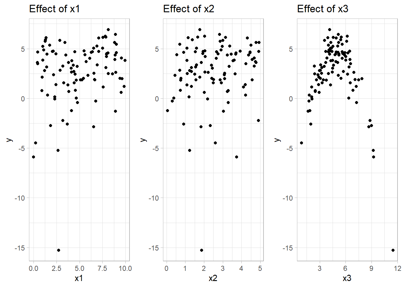
Figure 10.18: Scatter Plots of Variable Effects
# Fit a Regression Tree using rpart
tree_model <-
    rpart(
        y ~ x1 + x2 + x3,
        data = data_tree,
        method = "anova",
        control = rpart.control(cp = 0.01)
    )  # cp = complexity parameter

# Summary of the tree
summary(tree_model)
#> Call:
#> rpart(formula = y ~ x1 + x2 + x3, data = data_tree, method = "anova",
#>     control = rpart.control(cp = 0.01))
#>   n= 100
#>
#>           CP nsplit rel error    xerror      xstd
#> 1 0.39895879      0 1.0000000 1.0134781 0.3406703
#> 2 0.17470339      1 0.6010412 0.8649973 0.3336272
#> 3 0.04607373      2 0.4263378 0.5707932 0.1880333
#> 4 0.02754858      3 0.3802641 0.5287366 0.1866728
#> 5 0.01584638      4 0.3527155 0.5061104 0.1867491
#> 6 0.01032524      5 0.3368691 0.5136765 0.1861020
#> 7 0.01000000      7 0.3162187 0.4847072 0.1861849
#>
#> Variable importance
#> x3 x2 x1
#> 91  6  3
#>
#> Node number 1: 100 observations,    complexity param=0.3989588
#>   mean=2.639375, MSE=9.897038
#>   left son=2 (7 obs) right son=3 (93 obs)
#>   Primary splits:
#>       x3 < 7.707736  to the right, improve=0.39895880, (0 missing)
#>       x1 < 6.84138   to the left,  improve=0.07685517, (0 missing)
#>       x2 < 2.627429  to the left,  improve=0.04029839, (0 missing)
#>
#> Node number 2: 7 observations
#>   mean=-4.603469, MSE=24.47372
#>
#> Node number 3: 93 observations,    complexity param=0.1747034
#>   mean=3.184535, MSE=4.554158
#>   left son=6 (18 obs) right son=7 (75 obs)
#>   Primary splits:
#>       x3 < 2.967495  to the left,  improve=0.40823990, (0 missing)
#>       x2 < 1.001856  to the left,  improve=0.07353453, (0 missing)
#>       x1 < 6.84138   to the left,  improve=0.07049507, (0 missing)
#>   Surrogate splits:
#>       x2 < 0.3435293 to the left,  agree=0.828, adj=0.111, (0 split)
#>
#> Node number 6: 18 observations
#>   mean=0.4012593, MSE=3.4521
#>
#> Node number 7: 75 observations,    complexity param=0.04607373
#>   mean=3.852521, MSE=2.513258
#>   left son=14 (12 obs) right son=15 (63 obs)
#>   Primary splits:
#>       x3 < 6.324486  to the right, improve=0.24191360, (0 missing)
#>       x2 < 1.603258  to the left,  improve=0.10759280, (0 missing)
#>       x1 < 6.793804  to the left,  improve=0.09106168, (0 missing)
#>
#> Node number 14: 12 observations
#>   mean=2.065917, MSE=2.252311
#>
#> Node number 15: 63 observations,    complexity param=0.02754858
#>   mean=4.192826, MSE=1.839163
#>   left son=30 (9 obs) right son=31 (54 obs)
#>   Primary splits:
#>       x3 < 3.548257  to the left,  improve=0.2353119, (0 missing)
#>       x2 < 1.349633  to the left,  improve=0.1103019, (0 missing)
#>       x1 < 7.006669  to the left,  improve=0.1019295, (0 missing)
#>
#> Node number 30: 9 observations
#>   mean=2.581411, MSE=0.3669647
#>
#> Node number 31: 54 observations,    complexity param=0.01584638
#>   mean=4.461396, MSE=1.579623
#>   left son=62 (10 obs) right son=63 (44 obs)
#>   Primary splits:
#>       x2 < 1.130662  to the left,  improve=0.18386040, (0 missing)
#>       x1 < 6.209961  to the left,  improve=0.14561510, (0 missing)
#>       x3 < 4.517029  to the left,  improve=0.01044883, (0 missing)
#>
#> Node number 62: 10 observations
#>   mean=3.330957, MSE=2.001022
#>
#> Node number 63: 44 observations,    complexity param=0.01032524
#>   mean=4.718314, MSE=1.127413
#>   left son=126 (27 obs) right son=127 (17 obs)
#>   Primary splits:
#>       x1 < 6.468044  to the left,  improve=0.16079230, (0 missing)
#>       x3 < 5.608708  to the right, improve=0.05277854, (0 missing)
#>       x2 < 2.784688  to the left,  improve=0.03145241, (0 missing)
#>   Surrogate splits:
#>       x2 < 3.074905  to the left,  agree=0.636, adj=0.059, (0 split)
#>       x3 < 5.888028  to the left,  agree=0.636, adj=0.059, (0 split)
#>
#> Node number 126: 27 observations,    complexity param=0.01032524
#>   mean=4.380469, MSE=1.04313
#>   left son=252 (12 obs) right son=253 (15 obs)
#>   Primary splits:
#>       x1 < 3.658072  to the right, improve=0.4424566, (0 missing)
#>       x3 < 4.270123  to the right, improve=0.1430466, (0 missing)
#>       x2 < 2.658809  to the left,  improve=0.1121999, (0 missing)
#>   Surrogate splits:
#>       x2 < 2.707432  to the left,  agree=0.815, adj=0.583, (0 split)
#>       x3 < 4.010151  to the right, agree=0.593, adj=0.083, (0 split)
#>
#> Node number 127: 17 observations
#>   mean=5.25489, MSE=0.7920812
#>
#> Node number 252: 12 observations
#>   mean=3.620914, MSE=0.6204645
#>
#> Node number 253: 15 observations
#>   mean=4.988114, MSE=0.5504908
# Visualize the Regression Tree
rpart.plot(
tree_model,
type = 2,
extra = 101,
fallen.leaves = TRUE,
main = "Regression Tree"
)
Figure 2.7: Regression Tree
- Splits are made based on conditions (e.g., x1 < 4.2), partitioning the predictor space.
- Terminal nodes (leaves) show the predicted value (mean response in that region).
- The tree depth affects interpretability and overfitting risk.
# Optimal pruning based on cross-validation error
printcp(tree_model) # Displays CP table with cross-validation error
#>
#> Regression tree:
#> rpart(formula = y ~ x1 + x2 + x3, data = data_tree, method = "anova",
#>     control = rpart.control(cp = 0.01))
#>
#> Variables actually used in tree construction:
#> [1] x1 x2 x3
#>
#> Root node error: 989.7/100 = 9.897
#>
#> n= 100
#>
#>         CP nsplit rel error  xerror    xstd
#> 1 0.398959      0   1.00000 1.01348 0.34067
#> 2 0.174703      1   0.60104 0.86500 0.33363
#> 3 0.046074      2   0.42634 0.57079 0.18803
#> 4 0.027549      3   0.38026 0.52874 0.18667
#> 5 0.015846      4   0.35272 0.50611 0.18675
#> 6 0.010325      5   0.33687 0.51368 0.18610
#> 7 0.010000      7   0.31622 0.48471 0.18618
optimal_cp <-
    tree_model$cptable[which.min(tree_model$cptable[, "xerror"]), "CP"]

# Prune the tree
pruned_tree <- prune(tree_model, cp = optimal_cp)
# Visualize the pruned tree
rpart.plot(
pruned_tree,
type = 2,
extra = 101,
fallen.leaves = TRUE,
main = "Pruned Regression Tree"
)
Figure 2.9: Pruned Regression Tree Diagram
- Pruning reduces overfitting by simplifying the tree.
- The optimal CP minimizes cross-validation error, balancing complexity and fit.
- A shallower tree improves generalization on unseen data.
# Fit a Random Forest
set.seed(123)
rf_model <- randomForest(
    y ~ x1 + x2 + x3,
    data = data_tree,
    ntree = 500,
    mtry = 2,
    importance = TRUE
)

# Summary of the Random Forest
print(rf_model)
#>
#> Call:
#>  randomForest(formula = y ~ x1 + x2 + x3, data = data_tree, ntree = 500,      mtry = 2, importance = TRUE)
#>                Type of random forest: regression
#>                      Number of trees: 500
#> No. of variables tried at each split: 2
#>
#>           Mean of squared residuals: 3.031589
#> % Var explained: 69.37- MSE decreases as more trees are added.
- % Variance Explained reflects predictive performance.
mtry = 2indicates 2 random predictors are considered at each split.
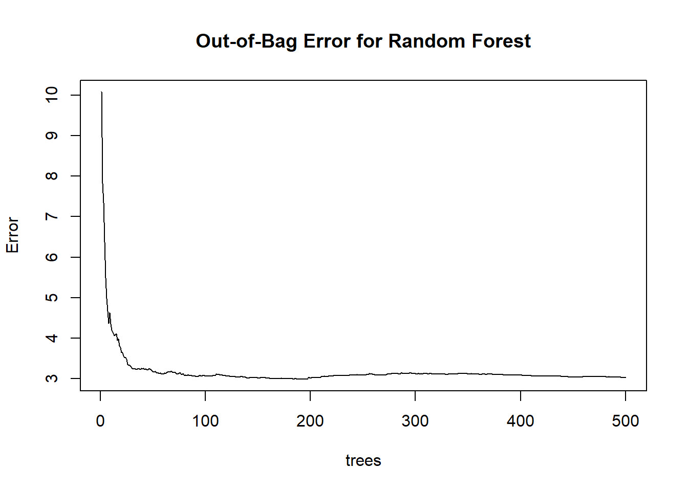
Figure 10.19: Out-of-Bag Error for Random Forest
- OOB error stabilizes as more trees are added, providing an unbiased estimate of test error.
- Helps determine if more trees improve performance or if the model has converged.
# Variable Importance
importance(rf_model)                # Numerical importance measures
#>      %IncMSE IncNodePurity
#> x1 10.145674     137.09918
#> x2  1.472662      77.41256
#> x3 44.232816     718.49567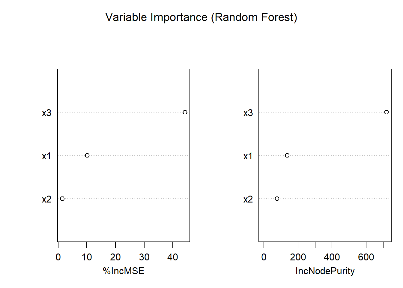
Figure 10.20: Variable Importance (Random Forest)
- Mean Decrease in MSE indicates how much the model’s error increases when a variable is permuted.
- Mean Decrease in Node Impurity reflects how much each variable reduces variance in splits.
- Variables with higher importance are more influential in the model.
# Predictions on new data
x_new <- seq(0, 10, length.out = 200)
test_data <- data.frame(x1 = x_new,
                        x2 = mean(x2),
                        x3 = mean(x3))

# Predictions
tree_pred <- predict(pruned_tree, newdata = test_data)
rf_pred <- predict(rf_model, newdata = test_data)
# Visualization
ggplot() +
geom_point(aes(x1, y),
data = data_tree,
alpha = 0.5,
color = "gray") +
geom_line(
aes(x_new, tree_pred),
color = "blue",
size = 1.2,
linetype = "dashed"
) +
geom_line(aes(x_new, rf_pred), color = "green", size = 1.2) +
labs(
title = "Regression Tree vs. Random Forest",
subtitle = "Blue: Pruned Tree | Green: Random Forest",
x = "x1",
y = "Predicted y"
) +
theme_minimal()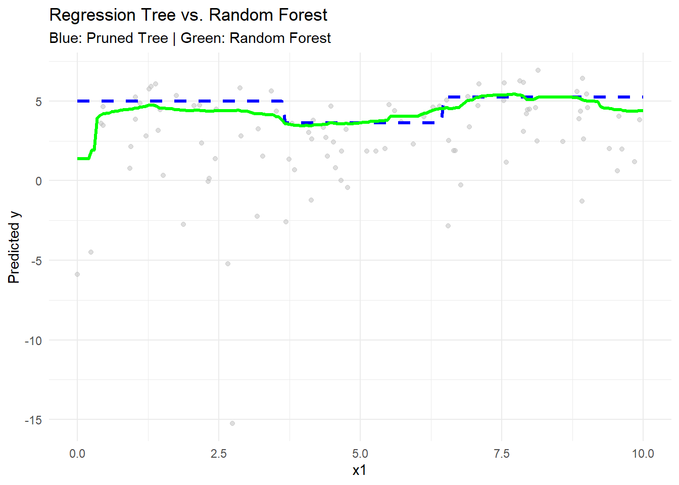
Figure 10.21: Regression Tree vs. Random Forest
- The pruned regression tree (blue) shows step-like predictions, characteristic of piecewise constant fits.
- The random forest (green) provides a smoother fit by averaging across many trees, reducing variance.
# OOB Error (Random Forest)
oob_mse <- rf_model$mse[length(rf_model$mse)]  # Final OOB MSE

# Cross-Validation Error (Regression Tree)
cv_mse_tree <-
    min(tree_model$cptable[, "xerror"]) * var(data_tree$y)

# Compare OOB and CV errors
data.frame(
    Model = c("Pruned Regression Tree", "Random Forest"),
    MSE = c(cv_mse_tree, oob_mse)
)
#>                    Model      MSE
#> 1 Pruned Regression Tree 4.845622
#> 2 Random Forest 3.031589- OOB error (Random Forest) provides an efficient, unbiased estimate without cross-validation.
- Cross-validation error (Regression Tree) evaluates generalization through resampling.
- Random Forest often shows lower MSE due to reduced variance.