34.5 Inference

Inference in IV models, particularly when instruments are weak, presents serious challenges that can undermine standard testing and confidence interval procedures. In this section, we explore the core issues of IV inference under weak instruments, discuss the standard and alternative approaches, and outline practical guidelines for applied research.

Consider the just-identified linear IV model:

$$Y = \beta X + u$$

where:

• $X$ is endogenous: $\text{Cov}(X, u) \neq 0$.

• $Z$ is an instrumental variable satisfying:

  • Relevance: $\text{Cov}(Z, X) \neq 0$.

  • Exogeneity: $\text{Cov}(Z, u) = 0$.

The IV estimator of $\beta$ is consistent under these assumptions.

A commonly used approach for inference is the t-ratio method, constructing a 95% confidence interval as:

$$\hat{\beta} \pm 1.96 \sqrt{\hat{V}_N(\hat{\beta})}$$

However, this approach is invalid when instruments are weak. Specifically:

• The t-ratio does not follow a standard normal distribution under weak instruments.

• Confidence intervals based on this method can severely under-cover the true parameter.

• Hypothesis tests can over-reject, even in large samples.

This problem was first systematically identified by Staiger and Stock (1997) and Dufour (1997). Weak instruments create distortions in the finite-sample distribution of $\hat{\beta}$.

Common Practices and Misinterpretations

1. Overreliance on t-Ratio Tests

• Popular but problematic when instruments are weak.
• Known to over-reject null hypotheses and under-cover confidence intervals.
• Documented extensively by Nelson and Startz (1990), Bound, Jaeger, and Baker (1995), Dufour (1997), and Lee et al. (2022).

2. Weak Instrument Diagnostics

• First-Stage F-Statistic:
  • Rule of thumb: $F > 10$ often used but simplistic and misleading.
  • More accurate critical values provided by J. H. Stock and Yogo (2005).
  • For 95% coverage, $F > 16.38$ is often cited (Staiger and Stock 1997).

3. Misinterpretations and Pitfalls

• Mistakenly interpreting $\hat{\beta} \pm 1.96 \times \hat{SE}$ as a 95% CI when the instrument is weak, Staiger and Stock (1997) show that under $F > 16.38$, the nominal 95% CI may only offer 85% coverage.
• Pretesting for weak instruments can exacerbate inference problems (A. R. Hall, Rudebusch, and Wilcox 1996).
• Selective model specification based on weak instrument diagnostics may introduce additional distortions (I. Andrews, Stock, and Sun 2019).

---

34.5.1 Weak Instruments Problem

An alternative statistic accounts for weak instrument issues by adjusting the standard Anderson-Rubin (AR) test:

$$\hat{t}^2 = \hat{t}^2_{AR} \times \frac{1}{1 - \hat{\rho} \frac{\hat{t}_{AR}}{\hat{f}} + \frac{\hat{t}^2_{AR}}{\hat{f}^2}}$$

Where:

• $\hat{t}^2_{AR} \sim \chi^2(1)$ under the null, even with weak instruments (T. W. Anderson and Rubin 1949).

• $\hat{t}_{AR} = \dfrac{\hat{\pi}(\hat{\beta} - \beta_0)}{\sqrt{\hat{V}_N (\hat{\pi} (\hat{\beta} - \beta_0))}} \sim N(0,1)$.

• $\hat{f} = \dfrac{\hat{\pi}}{\sqrt{\hat{V}_N(\hat{\pi})}}$ measures instrument strength (first-stage F-stat).

• $\hat{\pi}$ is the coefficient from the first-stage regression of $X$ on $Z$.

• $\hat{\rho} = \text{Cov}(Zv, Zu)$ captures the correlation between first-stage residuals and $u$.

Implications

• Even in large samples, $\hat{t}^2 \neq \hat{t}^2_{AR}$ because the adjustment term does not converge to zero unless instruments are strong and $\rho = 0$.
• The distribution of $\hat{t}$ does not match the standard normal but follows a more complex distribution described by Staiger and Stock (1997) and J. H. Stock and Yogo (2005).

---

The divergence between $\hat{t}^2$ and $\hat{t}^2_{AR}$ depends on:

1. Instrument Strength ($\pi$): Higher correlation between $Z$ and $X$ mitigates the problem.
2. First-Stage F-statistic ($E(F)$): A weak first-stage regression increases the bias and distortion.
3. Endogeneity Level ($|\rho|$): Greater correlation between $X$ and $u$ exacerbates inference errors.

---

Scenario	Conditions	Inference Quality
Worst Case	$\pi = 0$, $|\rho| = 1$	$\hat{\beta} \pm 1.96 \times SE$ fails; Type I error = 100%
Best Case	$\rho = 0$ (No endogeneity) or very large $\hat{f}$ (strong $Z$)	Standard inference works; intervals cover $\beta$ with correct rate
Intermediate Case	Moderate $\pi$, $\rho$, and $F$	Coverage and Type I error lie between extremes; standard inference risky

---

34.5.2 Solutions and Approaches for Valid Inference

1. Assume the Problem Away (Risky Assumptions)
   1. High First-Stage F-statistic:
      • Require $E(F) > 142.6$ for near-validity (Lee et al. 2022).
      • While the first-stage $F$ is observable, this threshold is high and often impractical.
   2. Low Endogeneity:
      • Assume $|\rho| < 0.565$ Lee et al. (2022). In other words, we assume endogeneity to be less than moderat level.
      • This undermines the motivation for IV in the first place, which exists precisely because of suspected endogeneity.
2. Confront the Problem Directly (Robust Methods)
   1. Anderson-Rubin (AR) Test (T. W. Anderson and Rubin 1949):
      • Valid under weak instruments.
      • Tests whether $Z$ explains variation in $Y - \beta_0 X$.
   2. tF Procedure (Lee et al. 2022):
      • Combines t-statistics and F-statistics in a unified testing framework.
      • Offers valid inference in presence of weak instruments.
   3. Andrews-Kolesár (AK) Procedure (J. Angrist and Kolesár 2023):
      • Provides uniformly valid confidence intervals for $\beta$.
      • Allows for weak instruments and arbitrary heteroskedasticity.
      • Especially useful in overidentified settings.

---

34.5.3 Anderson-Rubin Approach

The Anderson-Rubin (AR) test, originally proposed by T. W. Anderson and Rubin (1949), remains one of the most robust inferential tools in the context of instrumental variable estimation, particularly when instruments are weak or endogenous regressors exhibit complex error structures.

The AR test directly evaluates the joint null hypothesis that:

$$H_0: \beta = \beta_0$$

by testing whether the instruments explain any variation in the residuals $Y - \beta_0 X$. Under the null, the model becomes:

$$Y - \beta_0 X = u$$

Given that $\text{Cov}(Z, u) = 0$ (by the IV exogeneity assumption), the test regresses $(Y - \beta_0 X)$ on $Z$. The test statistic is constructed as:

$$AR(\beta_0) = \frac{(Y - \beta_0 X)' P_Z (Y - \beta_0 X)}{\hat{\sigma}^2}$$

• $P_Z$ is the projection matrix onto the column space of $Z$: $P_Z = Z (Z'Z)^{-1} Z'$.
• $\hat{\sigma}^2$ is an estimate of the error variance (under homoskedasticity).

Under $H_0$, the statistic follows a chi-squared distribution:

$$AR(\beta_0) \sim \chi^2(q)$$

where $q$ is the number of instruments (1 in a just-identified model).

---

Key Properties of the AR Test

• Robust to Weak Instruments:
  • The AR test does not rely on the strength of the instruments.
  • Its distribution under the null hypothesis remains valid even when the instruments are weak (Staiger and Stock 1997).
• Robust to Non-Normality and Homoskedastic Errors:
  • Maintains correct Type I error rates even under non-normal errors (Staiger and Stock 1997).
  • Optimality properties under homoskedastic errors are established in D. W. Andrews, Moreira, and Stock (2006) and M. J. Moreira (2009).
• Robust to Heteroskedasticity, Clustering, and Autocorrelation:
  • The AR test has been generalized to account for heteroskedasticity, clustered errors, and autocorrelation (J. H. Stock and Wright 2000; H. Moreira and Moreira 2019).
  • Valid inference is possible when combined with heteroskedasticity-robust variance estimators or cluster-robust techniques.

Setting	Validity	Reference
Non-Normal, Homoskedastic Errors	Valid without distributional assumptions	(Staiger and Stock 1997)
Heteroskedastic Errors	Generalized AR test remains valid; robust variance estimation recommended	(J. H. Stock and Wright 2000)
Clustered or Autocorrelated Errors	Extensions available using cluster-robust and HAC variance estimators	(H. Moreira and Moreira 2019)
Optimality under Homoskedasticity	AR test minimizes Type II error among invariant tests	(D. W. Andrews, Moreira, and Stock 2006; M. J. Moreira 2009)

---

The AR test is relatively simple to implement and is available in most econometric software. Here’s an intuitive step-by-step breakdown:

1. Specify the null hypothesis value $\beta_0$.
2. Compute the residual $u = Y - \beta_0 X$.
3. Regress $u$ on $Z$ and obtain the $R^2$ from this regression.
4. Compute the test statistic:

$$AR(\beta_0) = \frac{R^2 \cdot n}{q}$$

(For a just-identified model with a single instrument, $q=1$.)

5. Compare $AR(\beta_0)$ to the $\chi^2(q)$ distribution to determine significance.

library(ivDiag)

# AR test (robust to weak instruments)
# example by the package's authors
ivDiag::AR_test(
    data = rueda,
    Y = "e_vote_buying",
    # treatment
    D = "lm_pob_mesa",
    # instruments
    Z = "lz_pob_mesa_f",
    controls = c("lpopulation", "lpotencial"),
    cl = "muni_code",
    CI = FALSE
)
#> $Fstat
#>         F       df1       df2         p 
#>   48.4768    1.0000 4350.0000    0.0000

g <- ivDiag::ivDiag(
    data = rueda,
    Y = "e_vote_buying",
    D = "lm_pob_mesa",
    Z = "lz_pob_mesa_f",
    controls = c("lpopulation", "lpotencial"),
    cl = "muni_code",
    cores = 4,
    bootstrap = FALSE
)
g$AR
#> $Fstat
#>         F       df1       df2         p 
#>   48.4768    1.0000 4350.0000    0.0000 
#> 
#> $ci.print
#> [1] "[-1.2626, -0.7073]"
#> 
#> $ci
#> [1] -1.2626 -0.7073
#> 
#> $bounded
#> [1] TRUE
ivDiag::plot_coef(g)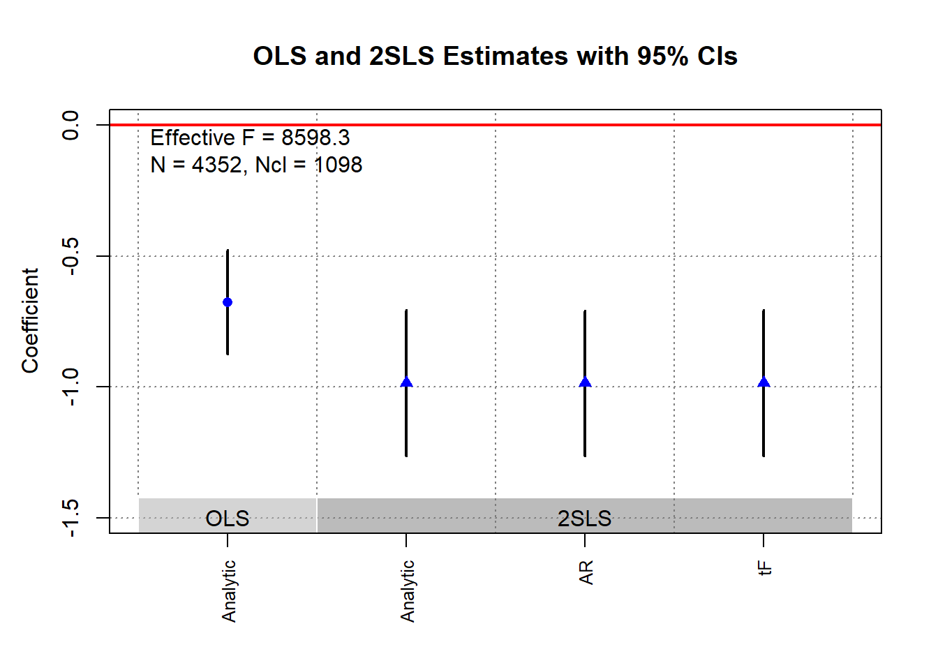

---

34.5.4 tF Procedure

Lee et al. (2022) introduce the tF procedure, an inference method specifically designed for just-identified IV models (single endogenous regressor and single instrument). It addresses the shortcomings of traditional 2SLS $t$-tests under weak instruments and offers a solution that is conceptually familiar to researchers trained in standard econometric practices.

Unlike the Anderson-Rubin test, which inverts hypothesis tests to form confidence sets, the tF procedure adjusts standard $t$-statistics and standard errors directly, making it a more intuitive extension of traditional hypothesis testing.

The tF procedure is widely applicable in settings where just-identified IV models arise, including:

• Randomized controlled trials with imperfect compliance
  (e.g., Local Average Treatment Effects in G. W. Imbens and Angrist (1994)).

• Fuzzy Regression Discontinuity Designs
  (e.g., Lee and Lemieux (2010)).

• Fuzzy Regression Kink Designs
  (e.g., (Card et al. 2015)).

A comparison of the AR approach and the tF procedure can be found in I. Andrews, Stock, and Sun (2019).

Feature	Anderson-Rubin	tF Procedure
Robustness to Weak IV	Yes (valid under weak instruments)	Yes (valid under weak instruments)
Finite Confidence Intervals	No (interval becomes infinite for $F \le 3.84$)	Yes (finite intervals for all $F$ values)
Interval Length	Often longer, especially when $F$ is moderate (e.g., $F = 16$)	Typically shorter than AR intervals for $F > 3.84$
Ease of Interpretation	Requires inverting tests; less intuitive	Directly adjusts $t$-based standard errors; more intuitive
Computational Simplicity	Moderate (inversion of hypothesis tests)	Simple (multiplicative adjustment to standard errors)

• With $F > 3.84$, the AR test’s expected interval length is infinite, whereas the tF procedure guarantees finite intervals, making it superior in practical applications with weak instruments.

The tF procedure adjusts the conventional 2SLS $t$-ratio for the first-stage F-statistic strength. Instead of relying on a pre-testing threshold (e.g., $F > 10$), the tF approach provides a smooth adjustment to the standard errors.

Key Features:

• Adjusts the 2SLS $t$-ratio based on the observed first-stage F-statistic.
• Applies different adjustment factors for different significance levels (e.g., 95% and 99%).
• Remains valid even when the instrument is weak, offering finite confidence intervals even when the first-stage F-statistic is low.

Advantages of the tF Procedure

1. Smooth Adjustment for First-Stage Strength

• The tF procedure smoothly adjusts inference based on the observed first-stage F-statistic, avoiding the need for arbitrary pre-testing thresholds (e.g., $F > 10$).

• It produces finite and usable confidence intervals even when the first-stage F-statistic is low:

  $$F > 3.84$$

• This threshold aligns with the critical value of 3.84 for a 95% Anderson-Rubin confidence interval, but with a crucial advantage:

  • The AR interval becomes unbounded (i.e., infinite length) when $F \le 3.84$.
  • The tF procedure, in contrast, still provides a finite confidence interval, making it more practical in weak instrument cases.

---

2. Clear and Interpretable Confidence Levels

• The tF procedure offers transparent confidence intervals that:

  • Directly incorporate the impact of first-stage instrument strength on the critical values used for inference.

  • Mirror the distortion-free properties of robust methods like the Anderson-Rubin test, but remain closer in spirit to conventional $t$-based inference.

• Researchers can interpret tF-based 95% and 99% confidence intervals using familiar econometric tools, without needing to invert hypothesis tests or construct confidence sets.

---

3. Robustness to Common Error Structures

• The tF procedure remains robust in the presence of:

  • Heteroskedasticity
  • Clustering
  • Autocorrelation

• No additional adjustments are necessary beyond the use of a robust variance estimator for both:

  • The first-stage regression
  • The second-stage IV regression

• As long as the same robust variance estimator is applied consistently, the tF adjustment maintains valid inference without imposing additional computational complexity.

---

4. Applicability to Published Research

• One of the most powerful features of the tF procedure is its flexibility for re-evaluating published studies:

  • Researchers only need the reported first-stage F-statistic and standard errors from the 2SLS estimates.

  • No access to the original data is required to recalculate confidence intervals or test statistical significance using the tF adjustment.

• This makes the tF procedure particularly valuable for meta-analyses, replications, and robustness checks of published IV studies, where:

  • Raw data may be unavailable, or
  • Replication costs are high.

---

Consider the linear IV model with additional covariates $W$:

$$Y = X \beta + W \gamma + u$$

$$X = Z \pi + W \xi + \nu$$

Where:

• $Y$: Outcome variable.

• $X$: Endogenous regressor of interest.

• $Z$: Instrumental variable (single instrument case).

• $W$: Vector of exogenous controls, possibly including an intercept.

• $u$, $\nu$: Error terms.

Key Statistics:

• $t$-ratio for the IV estimator:

  $$\hat{t} = \frac{\hat{\beta} - \beta_0}{\sqrt{\hat{V}_N (\hat{\beta})}}$$

• $t$-ratio for the first-stage coefficient:

  $$\hat{f} = \frac{\hat{\pi}}{\sqrt{\hat{V}_N (\hat{\pi})}}$$

• First-stage F-statistic:

  $$\hat{F} = \hat{f}^2$$

where

• $\hat{\beta}$: Instrumental variable estimator.
• $\hat{V}_N (\hat{\beta})$: Estimated variance of $\hat{\beta}$, possibly robust to deal with non-iid errors.
• $\hat{t}$: $t$-ratio under the null hypothesis.
• $\hat{f}$: $t$-ratio under the null hypothesis of $\pi=0$.

---

Under traditional asymptotics large samples, the $t$-ratio statistic follows:

$$\hat{t}^2 \to^d t^2$$

With critical values:

• $\pm 1.96$ for a 5% significance test.

• $\pm 2.58$ for a 1% significance test.

However, in IV settings (particularly with weak instruments):

• The distribution of the $t$-statistic is distorted (i.e., $t$-distribution might not be normal), even in large samples.

• The distortion arises because the strength of the instrument ($F$) and the degree of endogeneity ($\rho$) affect the $t$-distribution.

J. H. Stock and Yogo (2005) provide a formula to quantify this distortion (in the just-identified case) for Wald test statistics using 2SLS.:

$$t^2 = f + t_{AR} + \rho f t_{AR}$$

Where:

• $\hat{f} \to^d f$

• $\bar{f} = \dfrac{\pi}{\sqrt{\dfrac{1}{N} AV(\hat{\pi})}}$ and $AV(\hat{\pi})$ is the asymptotic variance of $\hat{\pi}$

• $t_{AR}$ is asymptotically standard normal ($AR = t^2_{AR}$)

• $\rho$ measures the correlation (degree of endogeneity) between $Zu$ and $Z\nu$ (when data are homoskedastic, $\rho$ is the correlation between $u$ and $\nu$).

Implications:

• For low $\rho$ ($\rho \in [0, 0.5]$), rejection probabilities can be below nominal levels.
• For high $\rho$ ($\rho = 0.8$), rejection rates can be inflated, e.g., 13% rejection at a nominal 5% significance level.
• Reliance on standard $t$-ratios leads to incorrect test sizes and invalid confidence intervals.

---

The tF procedure corrects for these distortions by adjusting the standard error of the 2SLS estimator based on the observed first-stage F-statistic.

Steps:

1. Estimate $\hat{\beta}$ and its conventional SE from 2SLS.
2. Compute the first-stage $\hat{F}$.
3. Multiply the conventional SE by an adjustment factor, which depends on $\hat{F}$ and the desired confidence level.
4. Compute new $t$-ratios and construct confidence intervals using standard critical values (e.g., $\pm 1.96$ for 95% CI).

Lee et al. (2022) refer to the adjusted standard errors as “0.05 tF SE” (for a 5% significance level) and “0.01 tF SE” (for 1%).

---

Lee et al. (2022) conducted a review of recent single-instrument studies in the American Economic Review.

Key Findings:

• For at least 25% of the examined specifications:
  • tF-adjusted confidence intervals were 49% longer at the 5% level.
  • tF-adjusted confidence intervals were 136% longer at the 1% level.
• Even among specifications with $F > 10$ and $t > 1.96$:
  • Approximately 25% became statistically insignificant at the 5% level after applying the tF adjustment.

Takeaway:

• The tF procedure can substantially alter inference conclusions.
• Published studies can be re-evaluated with the tF method using only the reported first-stage F-statistics, without requiring access to the underlying microdata.

---

library(ivDiag)
g <- ivDiag::ivDiag(
    data = rueda,
    Y = "e_vote_buying",
    D = "lm_pob_mesa",
    Z = "lz_pob_mesa_f",
    controls = c("lpopulation", "lpotencial"),
    cl = "muni_code",
    cores = 4,
    bootstrap = FALSE
)
g$tF
#>         F        cF      Coef        SE         t    CI2.5%   CI97.5%   p-value 
#> 8598.3264    1.9600   -0.9835    0.1424   -6.9071   -1.2626   -0.7044    0.0000

# example in fixest package
library(fixest)
library(tidyverse)
base = iris
names(base) = c("y", "x1", "x_endo_1", "x_inst_1", "fe")
set.seed(2)
base$x_inst_2 = 0.2 * base$y + 0.2 * base$x_endo_1 + rnorm(150, sd = 0.5)
base$x_endo_2 = 0.2 * base$y - 0.2 * base$x_inst_1 + rnorm(150, sd = 0.5)

est_iv = feols(y ~ x1 | x_endo_1 + x_endo_2 ~ x_inst_1 + x_inst_2, base)
est_iv
#> TSLS estimation - Dep. Var.: y
#>                   Endo.    : x_endo_1, x_endo_2
#>                   Instr.   : x_inst_1, x_inst_2
#> Second stage: Dep. Var.: y
#> Observations: 150
#> Standard-errors: IID 
#>              Estimate Std. Error  t value   Pr(>|t|)    
#> (Intercept)  1.831380   0.411435  4.45121 1.6844e-05 ***
#> fit_x_endo_1 0.444982   0.022086 20.14744  < 2.2e-16 ***
#> fit_x_endo_2 0.639916   0.307376  2.08186 3.9100e-02 *  
#> x1           0.565095   0.084715  6.67051 4.9180e-10 ***
#> ---
#> Signif. codes:  0 '***' 0.001 '**' 0.01 '*' 0.05 '.' 0.1 ' ' 1
#> RMSE: 0.398842   Adj. R2: 0.761653
#> F-test (1st stage), x_endo_1: stat = 903.2    , p < 2.2e-16 , on 2 and 146 DoF.
#> F-test (1st stage), x_endo_2: stat =   3.25828, p = 0.041268, on 2 and 146 DoF.
#>                   Wu-Hausman: stat =   6.79183, p = 0.001518, on 2 and 144 DoF.

res_est_iv <- est_iv$coeftable |> 
    rownames_to_column()


coef_of_interest <-
    res_est_iv[res_est_iv$rowname == "fit_x_endo_1", "Estimate"]
se_of_interest <-
    res_est_iv[res_est_iv$rowname == "fit_x_endo_1", "Std. Error"]
fstat_1st <- fitstat(est_iv, type = "ivf1")[[1]]$stat

# To get the correct SE based on 1st-stage F-stat (This result is similar without adjustment since F is large)
# the results are the new CIS and p.value
tF(coef = coef_of_interest, se = se_of_interest, Fstat = fstat_1st) |> 
    causalverse::nice_tab(5)
#>          F   cF  Coef     SE       t CI2.5. CI97.5. p.value
#> 1 903.1628 1.96 0.445 0.0221 20.1474 0.4017  0.4883       0

# We can try to see a different 1st-stage F-stat and how it changes the results
tF(coef = coef_of_interest, se = se_of_interest, Fstat = 2) |> 
    causalverse::nice_tab(5)
#>   F    cF  Coef     SE       t CI2.5. CI97.5. p.value
#> 1 2 18.66 0.445 0.0221 20.1474 0.0329  0.8571  0.0343

---

34.5.5 AK Approach

J. Angrist and Kolesár (2024) offer a reappraisal of just-identified IV models, focusing on the finite-sample properties of conventional inference in cases where a single instrument is used for a single endogenous variable. Their findings challenge some of the more pessimistic views about weak instruments and inference distortions in microeconometric applications.

Rather than propose a new estimator or test, Angrist and Kolesár provide a framework and rationale supporting the validity of traditional just-ID IV inference in many practical settings. Their insights clarify when conventional t-tests and confidence intervals can be trusted, and they offer practical guidance on first-stage pretesting, bias reduction, and endogeneity considerations.

AK apply their framework to three canonical studies:

1. J. D. Angrist and Krueger (1991) - Education returns
2. J. D. Angrist and Evans (1998) - Family size and female labor supply
3. J. D. Angrist and Lavy (1999) - Class size effects

Findings:

• Endogeneity ($\rho$) in these studies is moderate (typically $|\rho| < 0.47$).

• Conventional t-tests and confidence intervals work reasonably well.

• In many micro applications, theoretical bounds on causal effects and plausible OVB scenarios limit $\rho$, supporting the validity of conventional inference.

---

Key Contributions of the AK Approach

• Reassessing Bias and Coverage:
  AK demonstrate that conventional IV estimates and t-tests in just-ID IV models often perform better than theory might suggest—provided the degree of endogeneity ($\rho$) is moderate, and the first-stage F-statistic is not extremely weak.

• First-Stage Sign Screening:

  • They propose sign screening as a simple, costless strategy to halve the median bias of IV estimators.
  • Screening on the sign of the estimated first-stage coefficient (i.e., using only samples where the first-stage estimate has the correct sign) improves the finite-sample performance of just-ID IV estimates without degrading confidence interval coverage.

• Bias-Minimizing Screening Rule:

  • AK show that setting the first-stage t-statistic threshold $c = 0$, i.e., requiring only the correct sign of the first-stage estimate, minimizes median bias while preserving conventional coverage properties.

• Practical Implication:

  • They argue that conventional just-ID IV inference, including t-tests and confidence intervals, is likely valid in most microeconometric applications, especially where theory or institutional knowledge suggests the direction of the first-stage relationship.

---

34.5.5.1 Model Setup and Notation

AK adopt a reduced-form and first-stage specification for just-ID IV models:

$$Y_i = Z_i \delta + X_i' \psi_1 + u_i \\ D_i = Z_i \pi + X_i' \psi_2 + v_i$$

• $Y_i$: Outcome variable
• $D_i$: Endogenous treatment variable
• $Z_i$: Instrumental variable (single instrument)
• $X_i$: Control variables
• $u_i, v_i$: Error terms

Parameter of Interest:

$$\beta = \frac{\delta}{\pi}$$

---

34.5.5.2 Endogeneity and Instrument Strength

AK characterize the two key parameters governing finite-sample inference:

• Instrument Strength:
  $$E[F] = \frac{\pi^2}{\sigma^2_{\hat{\pi}}} + 1$$
  (Expected value of the first-stage F-statistic.)

• Endogeneity:
  $$\rho = \text{cor}(\hat{\delta} - \hat{\pi} \beta, \hat{\pi})$$
  Measures the degree of correlation between reduced-form and first-stage residuals (or between $u$ and $v$ under homoskedasticity).

Key Insight:

For $\rho < 0.76$, the coverage of conventional 95% confidence intervals is distorted by less than 5%, regardless of the first-stage F-statistic.

---

34.5.5.3 First-Stage Sign Screening

AK argue that pre-screening based on the sign of the first-stage estimate ($\hat{\pi}$) offers bias reduction without compromising confidence interval coverage.

Screening Rule:

• Screen if $\hat{\pi} > 0$
  (or $\hat{\pi} < 0$ if the theoretical sign is negative).

Results:

• Halves median bias of the IV estimator.
• No degradation of confidence interval coverage.

This screening approach:

• Avoids the pitfalls of pre-testing based on first-stage F-statistics (which can exacerbate bias and distort inference).

• Provides a “free lunch”: bias reduction with no coverage cost.

---

34.5.5.4 Rejection Rates and Confidence Interval Coverage

• Rejection rates of conventional t-tests stay close to the nominal level (5%) if $|\rho| < 0.76$, independent of instrument strength.
• For $|\rho| < 0.565$, conventional t-tests exhibit no over-rejection, aligning with findings from Lee et al. (2022).

Comparison with AR and tF Procedures:

Approach	Bias Reduction	Coverage	CI Length (F > 3.84)
AK Sign Screening	Halves median bias	Near-nominal	Finite
AR Test	No bias (inversion method)	Exact	Infinite
tF Procedure	Bias adjusted	Near-nominal	Longer than AK (especially for moderate F)

---

References

Anderson, Theodore W, and Herman Rubin. 1949. “Estimation of the Parameters of a Single Equation in a Complete System of Stochastic Equations.” The Annals of Mathematical Statistics 20 (1): 46–63.

Andrews, Donald WK, Marcelo J Moreira, and James H Stock. 2006. “Optimal Two-Sided Invariant Similar Tests for Instrumental Variables Regression.” Econometrica 74 (3): 715–52.

Andrews, Isaiah, James H Stock, and Liyang Sun. 2019. “Weak Instruments in Instrumental Variables Regression: Theory and Practice.” Annual Review of Economics 11: 727–53.

Angrist, Joshua D, and William N Evans. 1998. “Children and Their Parents’ Labor Supply: Evidence from Exogenous Variation in Family Size.” American Economic Review 88 (3).

Angrist, Joshua D, and Alan B Krueger. 1991. “Does Compulsory School Attendance Affect Schooling and Earnings?” The Quarterly Journal of Economics 106 (4): 979–1014.

Angrist, Joshua D, and Victor Lavy. 1999. “Using Maimonides’ Rule to Estimate the Effect of Class Size on Scholastic Achievement.” The Quarterly Journal of Economics 114 (2): 533–75.

Angrist, Joshua, and Michal Kolesár. 2023. “One Instrument to Rule Them All: The Bias and Coverage of Just-ID IV.” Journal of Econometrics.

———. 2024. “One Instrument to Rule Them All: The Bias and Coverage of Just-ID IV.” Journal of Econometrics 240 (2): 105398.

Bound, John, David A Jaeger, and Regina M Baker. 1995. “Problems with Instrumental Variables Estimation When the Correlation Between the Instruments and the Endogenous Explanatory Variable Is Weak.” Journal of the American Statistical Association 90 (430): 443–50.

Card, David, David S Lee, Zhuan Pei, and Andrea Weber. 2015. “Inference on Causal Effects in a Generalized Regression Kink Design.” Econometrica 83 (6): 2453–83.

Dufour, Jean-Marie. 1997. “Some Impossibility Theorems in Econometrics with Applications to Structural and Dynamic Models.” Econometrica: Journal of the Econometric Society, 1365–87.

Hall, Alastair R, Glenn D Rudebusch, and David W Wilcox. 1996. “Judging Instrument Relevance in Instrumental Variables Estimation.” International Economic Review, 283–98.

Imbens, Guido W, and Joshua D Angrist. 1994. “Identification and Estimation of Local Average Treatment Effects.” Econometrica 62 (2): 467–75.

Lee, David S, and Thomas Lemieux. 2010. “Regression Discontinuity Designs in Economics.” Journal of Economic Literature 48 (2): 281–355.

Lee, David S, Justin McCrary, Marcelo J Moreira, and Jack Porter. 2022. “Valid t-Ratio Inference for IV.” American Economic Review 112 (10): 3260–90.

Moreira, Humberto, and Marcelo J Moreira. 2019. “Optimal Two-Sided Tests for Instrumental Variables Regression with Heteroskedastic and Autocorrelated Errors.” Journal of Econometrics 213 (2): 398–433.

———. 2009. “Tests with Correct Size When Instruments Can Be Arbitrarily Weak.” Journal of Econometrics 152 (2): 131–40.

Nelson, Charles R, and Richard Startz. 1990. “The Distribution of the Instrumental Variables Estimator and Its t-Ratio When the Instrument Is a Poor One.” Journal of Business, S125–40.

Staiger, Douglas, and James H Stock. 1997. “Instrumental Variables Regression with Weak Instruments.” Econometrica 65 (3): 557–86.

Stock, James H, and Jonathan H Wright. 2000. “GMM with Weak Identification.” Econometrica 68 (5): 1055–96.

———. 2005. “Testing for Weak Instruments in Linear IV Regression.” Identification and Inference for Econometric Models: Essays in Honor of Thomas Rothenberg, 80.