39.1 Bad Controls

39.1.1 M-bias

A common intuition in causal inference is to control for any variable that precedes the treatment. This logic underpins much of the guidance in traditional econometric texts (G. W. Imbens and Rubin 2015; J. D. Angrist and Pischke 2009), where pre-treatment variables like $Z$ are often recommended as controls if they correlate with both the treatment $X$ and the outcome $Y$.

This perspective is especially prevalent in Matching Methods, where all observed pre-treatment covariates are typically included in the matching process. However, controlling for every pre-treatment variable can lead to bad control bias.

One such example is M-bias, which arises when conditioning on a collider — a variable that is influenced by two unobserved causes. The DAG below illustrates a case where $Z$ appears to be a good control but actually opens a biasing path:

# Clean workspace
rm(list = ls())

# DAG specification
model <- dagitty("dag{
  x -> y
  u1 -> x
  u1 -> z
  u2 -> z
  u2 -> y
}")

# Set latent variables
latents(model) <- c("u1", "u2")

# Coordinates for plotting
coordinates(model) <- list(
  x = c(x = 1, u1 = 1, z = 2, u2 = 3, y = 3),
  y = c(x = 1, u1 = 2, z = 1.5, u2 = 2, y = 1)
)

# Plot the DAG
ggdag(model) + theme_dag()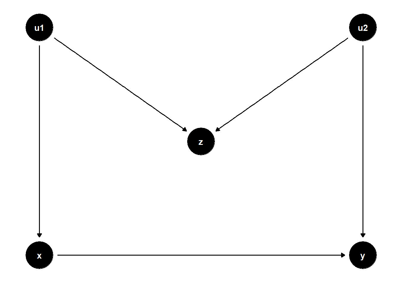

In this structure, $Z$ is a collider on the path $X \leftarrow U_1 \rightarrow Z \leftarrow U_2 \rightarrow Y$. Controlling for $Z$ opens this path, introducing a spurious association between $X$ and $Y$ even if none existed originally.

Even though $Z$ is statistically correlated with both $X$ and $Y$, it is not a confounder, because it does not lie on a back-door path that needs to be blocked. Instead, adjusting for $Z$ biases the estimate of the causal effect of $X \to Y$.

Let’s illustrate this with a simulation:

set.seed(123)

n <- 1e4
u1 <- rnorm(n)
u2 <- rnorm(n)
z <- u1 + u2 + rnorm(n)
x <- u1 + rnorm(n)
causal_coef <- 2
y <- causal_coef * x - 4 * u2 + rnorm(n)

# Compare unadjusted and adjusted models
jtools::export_summs(
  lm(y ~ x),
  lm(y ~ x + z),
  model.names = c("Unadjusted", "Adjusted")
)

	Unadjusted	Adjusted
(Intercept)	0.05	0.03
	(0.04)	(0.03)
x	2.01 ***	2.80 ***
	(0.03)	(0.03)
z		-1.57 ***
		(0.02)
N	10000	10000
R2	0.32	0.57
*** p < 0.001; ** p < 0.01; * p < 0.05.

Notice how adjusting for $Z$ changes the estimate of the effect of $X$ on $Y$, even though $Z$ is not a true confounder. This is a textbook example of M-bias in practice.

39.1.1.1 Worse: M-bias with Direct Effect from Z to Y

A more difficult case arises when $Z$ also has a direct effect on $Y$. Consider the DAG below:

# Clean workspace
rm(list = ls())

# DAG specification
model <- dagitty("dag{
  x -> y
  u1 -> x
  u1 -> z
  u2 -> z
  u2 -> y
  z -> y
}")

# Set latent variables
latents(model) <- c("u1", "u2")

# Coordinates for plotting
coordinates(model) <- list(
  x = c(x = 1, u1 = 1, z = 2, u2 = 3, y = 3),
  y = c(x = 1, u1 = 2, z = 1.5, u2 = 2, y = 1)
)

# Plot the DAG
ggdag(model) + theme_dag()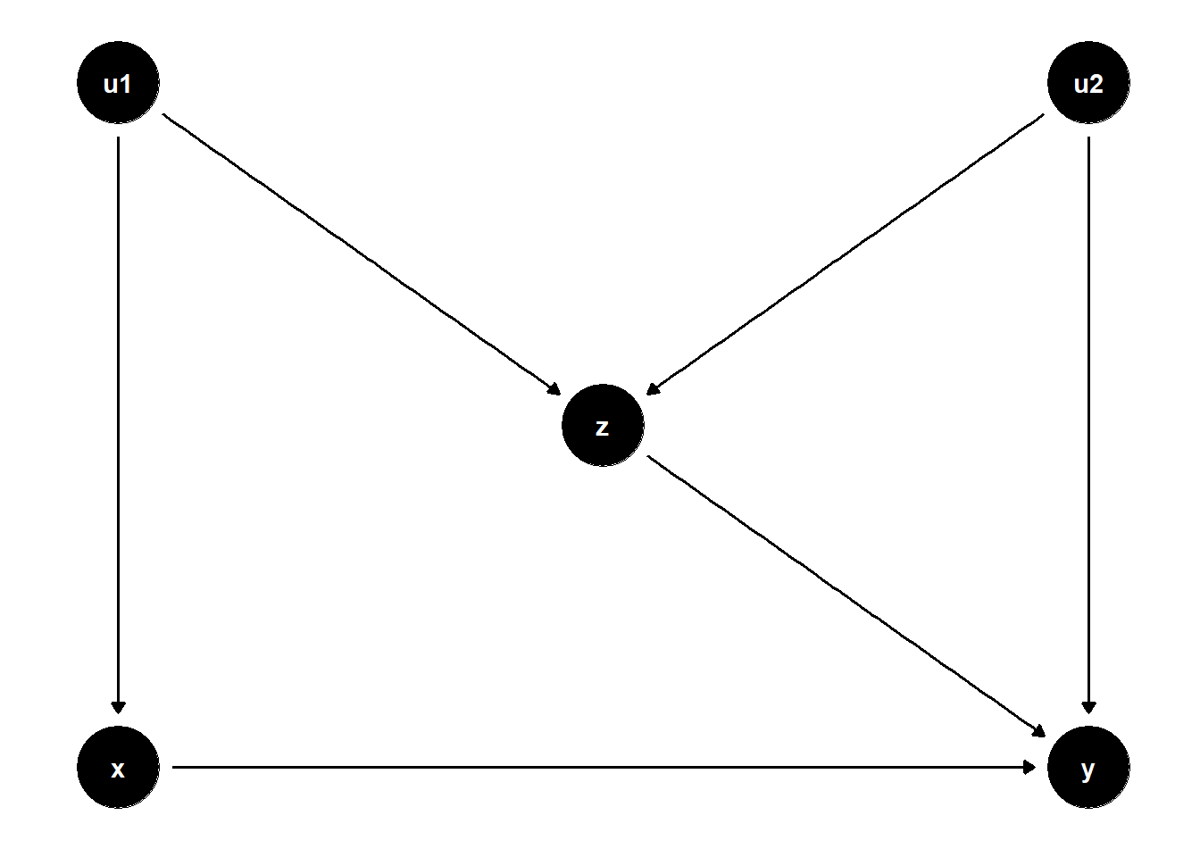

This situation presents a dilemma:

• Not controlling for $Z$ leaves the back-door path $X \leftarrow U_1 \to Z \to Y$ open, introducing confounding bias.

• Controlling for $Z$ opens the collider path $X \leftarrow U_1 \to Z \leftarrow U_2 \to Y$, which also biases the estimate.

In short, no adjustment strategy can fully remove bias from the estimate of $X \to Y$ using observed data alone.

What Can Be Done?

When facing such situations, we often turn to sensitivity analysis to assess how robust our causal conclusions are to unmeasured confounding. Specifically, recent advances (Cinelli et al. 2019; Cinelli and Hazlett 2020) allow us to quantify:

1. Plausible bounds on the strength of the direct effect $Z \to Y$

2. Sensitivity parameters reflecting the possible influence of the latent variables $U_1$ and $U_2$

These tools help us understand how large the unmeasured biases would have to be in order to overturn our conclusions — a pragmatic approach when perfect control is impossible.

39.1.2 Bias Amplification

Bias amplification occurs when controlling for a variable that is not a confounder — in fact, controlling for it increases bias due to an unobserved confounder.

In the DAG below, $U$ is an unobserved common cause of both $X$ and $Y$. $Z$ influences $X$ but has no causal relationship with $Y$. Including $Z$ in the model does not block any back-door path but instead increases the bias from $U$ by amplifying its association with $X$.

# Clean workspace
rm(list = ls())

# DAG specification
model <- dagitty("dag{
  x -> y
  u -> x
  u -> y
  z -> x
}")

# Set latent variable
latents(model) <- c("u")

# Coordinates for plotting
coordinates(model) <- list(
  x = c(z = 1, x = 2, u = 3, y = 4),
  y = c(z = 1, x = 1, u = 2, y = 1)
)

# Plot the DAG
ggdag(model) + theme_dag()

Even though $Z$ is a strong predictor of $X$, it is not a confounder, because it is not a common cause of $X$ and $Y$. Controlling for $Z$ increases the portion of $X$’s variation explained by $U$, thus amplifying bias in estimating the effect of $X$ on $Y$.

Simulation:

set.seed(123)
n <- 1e4
z <- rnorm(n)
u <- rnorm(n)
x <- 2*z + u + rnorm(n)
y <- x + 2*u + rnorm(n)

jtools::export_summs(
  lm(y ~ x),
  lm(y ~ x + z),
  model.names = c("Unadjusted", "Adjusted")
)

	Unadjusted	Adjusted
(Intercept)	-0.02	-0.01
	(0.02)	(0.02)
x	1.32 ***	1.99 ***
	(0.01)	(0.01)
z		-2.01 ***
		(0.03)
N	10000	10000
R2	0.71	0.80
*** p < 0.001; ** p < 0.01; * p < 0.05.

Observe that the adjusted model is more biased than the unadjusted one. This illustrates how controlling for a variable like $Z$ can amplify omitted variable bias.

39.1.3 Overcontrol Bias

Overcontrol bias arises when we adjust for variables that lie on the causal path from treatment to outcome, or that serve as proxies for the outcome.

39.1.3.1 Mediator Control

Controlling for a mediator — a variable that lies on the causal path between treatment and outcome — removes part of the effect we are trying to estimate.

# Clean workspace
rm(list = ls())

# DAG: X → Z → Y
model <- dagitty("dag{
  x -> z
  z -> y
}")

coordinates(model) <- list(
  x = c(x = 1, z = 2, y = 3),
  y = c(x = 1, z = 1, y = 1)
)

ggdag(model) + theme_dag()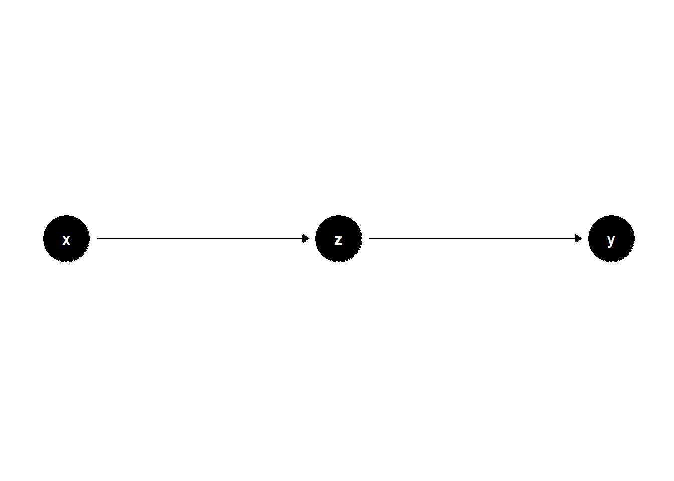

If we want to estimate the total effect of $X$ on $Y$, controlling for $Z$ (a mediator) leads to overcontrol bias.

set.seed(123)
n <- 1e4
x <- rnorm(n)
z <- x + rnorm(n)
y <- z + rnorm(n)

jtools::export_summs(
  lm(y ~ x),
  lm(y ~ x + z),
  model.names = c("Total Effect", "Controlled for Mediator")
)

	Total Effect	Controlled for Mediator
(Intercept)	-0.02	-0.01
	(0.01)	(0.01)
x	1.03 ***	0.02
	(0.01)	(0.01)
z		1.00 ***
		(0.01)
N	10000	10000
R2	0.34	0.67
*** p < 0.001; ** p < 0.01; * p < 0.05.

Here, $Z$ will appear significant, but including it blocks the causal path from $X$ to $Y$. This is misleading when the goal is to estimate the total effect of $X$.

39.1.3.2 Proxy for Mediator

In more complex scenarios, controlling for variables that proxy for mediators can introduce similar distortions.

# Clean workspace
rm(list = ls())

# DAG: X → M → Z, M → Y
model <- dagitty("dag{
  x -> m
  m -> z
  m -> y
}")

coordinates(model) <- list(
  x = c(x = 1, m = 2, z = 2, y = 3),
  y = c(x = 2, m = 2, z = 1, y = 2)
)

ggdag(model) + theme_dag()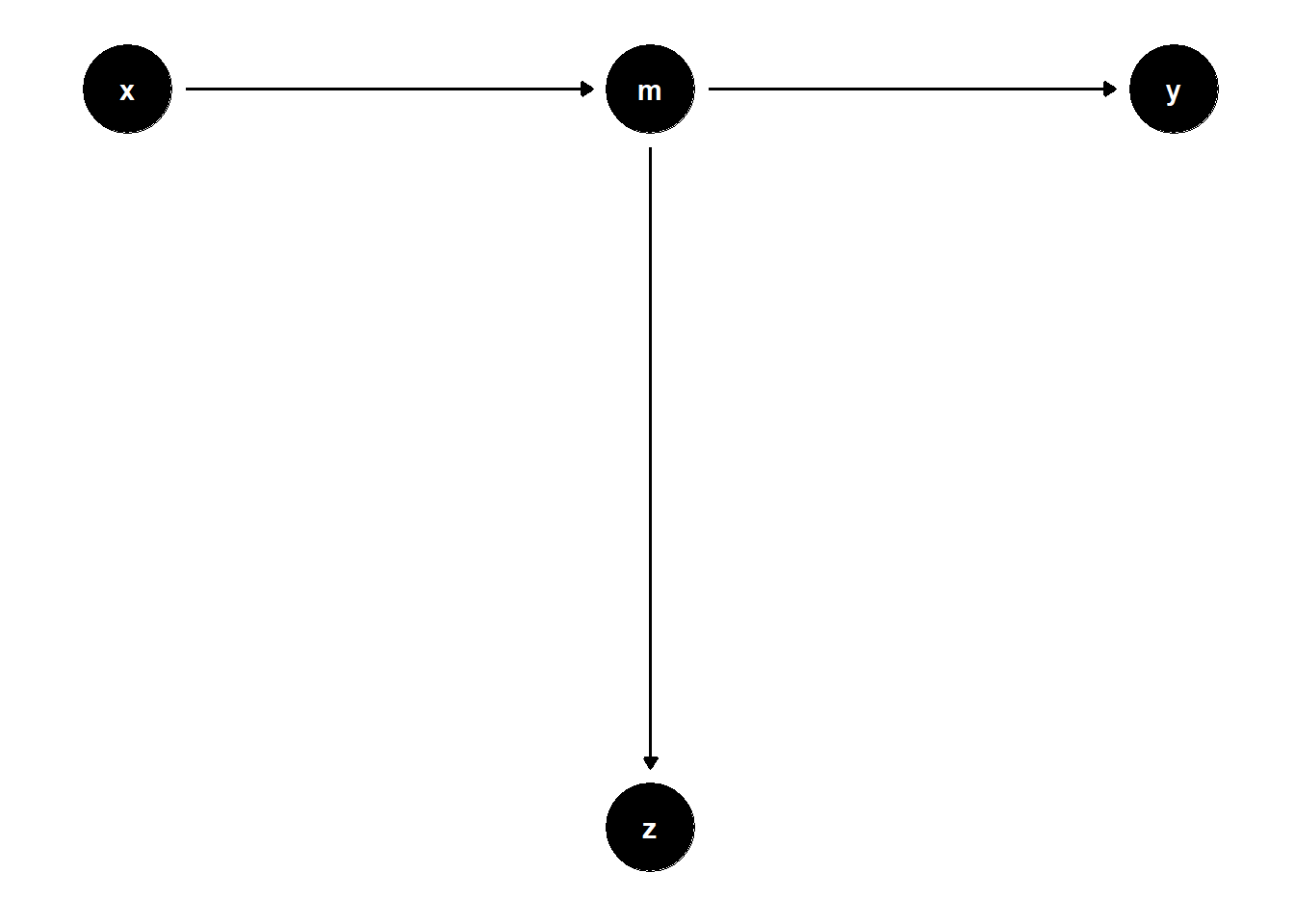

set.seed(123)
n <- 1e4
x <- rnorm(n)
m <- x + rnorm(n)
z <- m + rnorm(n)
y <- m + rnorm(n)


jtools::export_summs(lm(y ~ x),
                     lm(y ~ x + z),
                     model.names = c("Total Effect", "Controlled for Proxy Z"))

	Total Effect	Controlled for Proxy Z
(Intercept)	-0.01	-0.01
	(0.01)	(0.01)
x	0.99 ***	0.49 ***
	(0.01)	(0.02)
z		0.49 ***
		(0.01)
N	10000	10000
R2	0.33	0.49
*** p < 0.001; ** p < 0.01; * p < 0.05.

Even though $Z$ is not on the path from $X$ to $Y$, controlling for it removes part of the causal variation coming through $M$.

39.1.3.3 Overcontrol with Unobserved Confounding

When $Z$ is influenced by both $X$ and a latent confounder $U$ that also affects $Y$, controlling for $Z$ again biases the estimate.

# Clean workspace
rm(list = ls())

# DAG: X → Z → Y; U → Z, U → Y
model <- dagitty("dag{
  x -> z
  z -> y
  u -> z
  u -> y
}")

latents(model) <- "u"

coordinates(model) <- list(
  x = c(x = 1, z = 2, u = 3, y = 4),
  y = c(x = 1, z = 1, u = 2, y = 1)
)

ggdag(model) + theme_dag()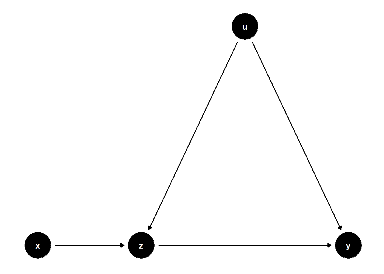

set.seed(1)
n <- 1e4
x <- rnorm(n)
u <- rnorm(n)
z <- x + u + rnorm(n)
y <- z + u + rnorm(n)

jtools::export_summs(
  lm(y ~ x),
  lm(y ~ x + z),
  model.names = c("Unadjusted", "Controlled for Z")
)

	Unadjusted	Controlled for Z
(Intercept)	-0.01	-0.01
	(0.02)	(0.01)
x	1.01 ***	-0.47 ***
	(0.02)	(0.01)
z		1.48 ***
		(0.01)
N	10000	10000
R2	0.15	0.78
*** p < 0.001; ** p < 0.01; * p < 0.05.

Although the total effect of $X$ on $Y$ is correctly captured in the unadjusted model, adjusting for $Z$ introduces bias via the collider path $X \to Z \leftarrow U \to Y$.

Insight: Controlling for $Z$ inadvertently blocks the direct effect of $X$ and opens a biasing path through $U$. This makes the adjusted model unreliable for causal inference.

These examples highlight the importance of conceptual clarity and causal reasoning in model specification. Not all covariates should be controlled for — especially not those that are:

• Mediators (on the causal path)

• Proxies for mediators or outcomes

• Colliders or descendants of colliders

In business contexts, this often arises when analysts include intermediate variables like sales leads, customer engagement scores, or operational metrics without understanding whether these mediate the effect of a treatment (e.g., ad spend) or confound it.

39.1.4 Selection Bias

Selection bias — also known as collider stratification bias — occurs when conditioning on a variable that is a collider (a common effect of two or more variables). This inadvertently opens non-causal paths, inducing spurious associations between variables that are otherwise independent or unconfounded.

39.1.4.1 Classic Collider Bias

In the DAG below, $Z$ is a collider between $X$ and a latent variable $U$. Controlling for $Z$ opens a back-door path from $X$ to $Y$ through $U$, introducing bias.

rm(list = ls())

# DAG
model <- dagitty("dag{
  x -> y
  x -> z
  u -> z
  u -> y
}")
latents(model) <- "u"
coordinates(model) <- list(
  x = c(x = 1, z = 2, u = 2, y = 3),
  y = c(x = 3, z = 2, u = 4, y = 3)
)
ggdag(model) + theme_dag()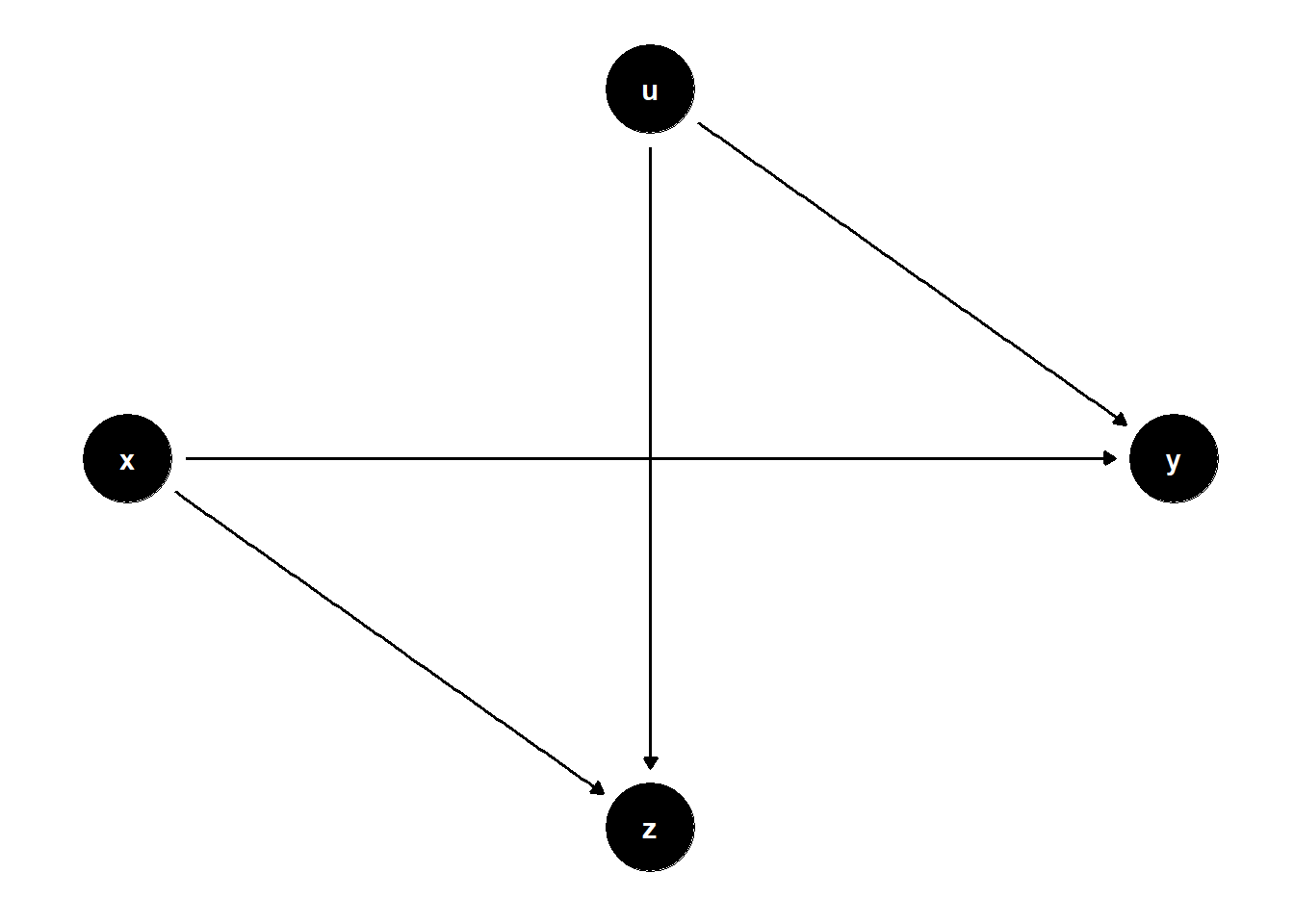

Simulation:

set.seed(123)
n <- 1e4
x <- rnorm(n)
u <- rnorm(n)
z <- x + u + rnorm(n)
y <- x + 2*u + rnorm(n)

jtools::export_summs(
  lm(y ~ x),
  lm(y ~ x + z),
  model.names = c("Unadjusted", "Adjusted for Z (collider)")
)

	Unadjusted	Adjusted for Z (collider)
(Intercept)	-0.02	-0.01
	(0.02)	(0.02)
x	0.99 ***	-0.02
	(0.02)	(0.02)
z		0.99 ***
		(0.01)
N	10000	10000
R2	0.17	0.49
*** p < 0.001; ** p < 0.01; * p < 0.05.

Controlling for $Z$ opens the non-causal path $X \to Z \leftarrow U \to Y$, resulting in biased estimates of the effect of $X$ on $Y$.

39.1.4.2 Collider Between Treatment and Outcome

In some cases, the collider is influenced directly by both the treatment and the outcome. This setting is also highly relevant in observational designs, particularly in retrospective or convenience sampling scenarios.

rm(list = ls())

# DAG: X → Z ← Y
model <- dagitty("dag{
  x -> y
  x -> z
  y -> z
}")
coordinates(model) <- list(
  x = c(x = 1, z = 2, y = 3),
  y = c(x = 2, z = 1, y = 2)
)
ggdag(model) + theme_dag()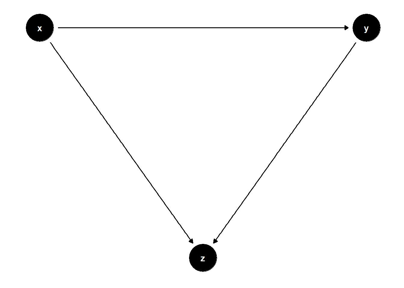

Simulation:

set.seed(123)
n <- 1e4
x <- rnorm(n)
y <- x + rnorm(n)
z <- x + y + rnorm(n)

jtools::export_summs(
  lm(y ~ x),
  lm(y ~ x + z),
  model.names = c("Unadjusted", "Adjusted for Collider Z")
)

	Unadjusted	Adjusted for Collider Z
(Intercept)	-0.01	-0.00
	(0.01)	(0.01)
x	1.01 ***	-0.01
	(0.01)	(0.01)
z		0.50 ***
		(0.01)
N	10000	10000
R2	0.50	0.75
*** p < 0.001; ** p < 0.01; * p < 0.05.

Even though $Z$ is associated with both $X$ and $Y$, it should not be controlled for, because doing so opens the collider path $X \to Z \leftarrow Y$, generating spurious dependence.

39.1.5 Case-Control Bias

Case-control studies often condition on the outcome (or its descendants), which can lead to collider bias if not properly accounted for.

In the DAG below, $Z$ is a descendant of a collider. Controlling for it can again induce spurious correlations by opening non-causal paths.

rm(list = ls())

# DAG: X → Y → Z
model <- dagitty("dag{
  x -> y
  y -> z
}")
coordinates(model) <- list(
  x = c(x = 1, z = 2, y = 3),
  y = c(x = 2, z = 1, y = 2)
)
ggdag(model) + theme_dag()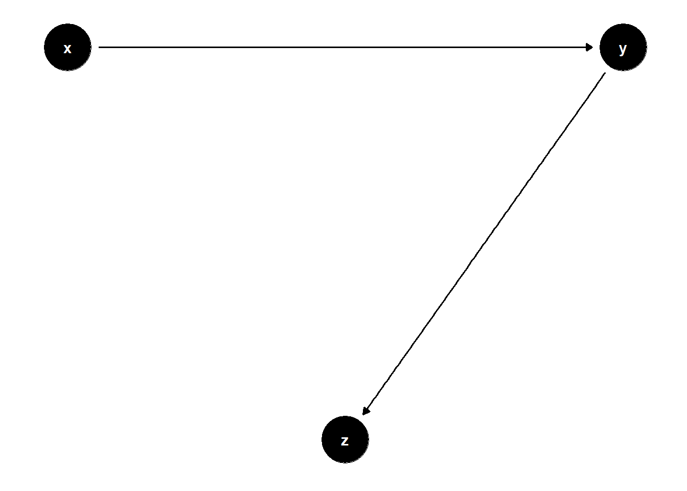

Simulation:

set.seed(123)
n <- 1e4
x <- rnorm(n)
y <- x + rnorm(n)
z <- y + rnorm(n)

jtools::export_summs(
  lm(y ~ x),
  lm(y ~ x + z),
  model.names = c("Unadjusted", "Adjusted for Descendant Z")
)

	Unadjusted	Adjusted for Descendant Z
(Intercept)	-0.01	-0.00
	(0.01)	(0.01)
x	1.01 ***	0.49 ***
	(0.01)	(0.01)
z		0.50 ***
		(0.01)
N	10000	10000
R2	0.50	0.75
*** p < 0.001; ** p < 0.01; * p < 0.05.

Note the subtlety: if $X$ has a true causal effect on $Y$, then controlling for $Z$ biases the estimate. However, if $X$ has no causal effect on $Y$, then $X$ is d-separated from $Y$, even when adjusting for $Z$. In that special case, controlling for $Z$ will not falsely suggest an effect.

Key Insight: Whether or not adjustment induces bias depends on the presence or absence of a true causal path. This highlights the importance of DAGs in clarifying assumptions and guiding valid statistical inference.

39.1.6 Summary

Bias Type	Key Mistake	Path Opened	Consequence
M-Bias	Controlling for a collider	$X \leftarrow U_1 \to Z \leftarrow U_2 \to Y$	Spurious association
Bias Amplification	Controlling for a non-confounder	Amplifies unobserved confounding	Larger bias than before
Overcontrol Bias	Controlling for a mediator or proxy	Blocks part of causal effect	Underestimates total effect
Selection Bias	Conditioning on a collider or its descendant	$X \to Z \leftarrow Y$ or similar	Induced non-causal correlation
Case-Control Bias	Conditioning on a variable affected by outcome	$X \to Y \to Z$	Collider-induced associatio

---

References

Angrist, Joshua D, and Jörn-Steffen Pischke. 2009. Mostly Harmless Econometrics: An Empiricist’s Companion. Princeton university press.

Cinelli, Carlos, and Chad Hazlett. 2020. “Making Sense of Sensitivity: Extending Omitted Variable Bias.” Journal of the Royal Statistical Society Series B: Statistical Methodology 82 (1): 39–67.

Cinelli, Carlos, Daniel Kumor, Bryant Chen, Judea Pearl, and Elias Bareinboim. 2019. “Sensitivity Analysis of Linear Structural Causal Models.” In International Conference on Machine Learning, 1252–61. PMLR; Proceedings of Machine Learning Research.

Imbens, Guido W, and Donald B Rubin. 2015. Causal Inference in Statistics, Social, and Biomedical Sciences. Cambridge University Press.