41.3 Missing Data

Missingness is information. First detect, then decide: delete, impute, or model it explicitly.

# Counts by variable
profile_missing(tx)
#> # A tibble: 13 × 3
#>    feature    num_missing pct_missing
#>    <fct>            <int>       <dbl>
#>  1 city                 0      0     
#>  2 year                 0      0     
#>  3 month                0      0     
#>  4 sales              568      0.0660
#>  5 volume             568      0.0660
#>  6 median             616      0.0716
#>  7 listings          1424      0.166 
#>  8 inventory         1467      0.171 
#>  9 date                 0      0     
#> 10 avg_price          568      0.0660
#> 11 absorption        1427      0.166 
#> 12 quarter              0      0     
#> 13 ym                   0      0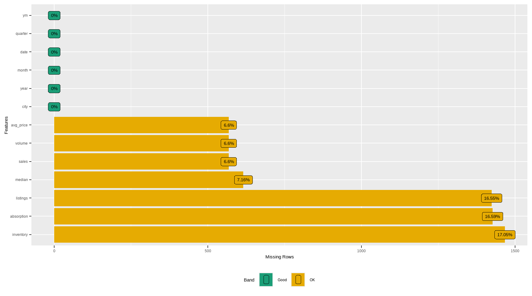

plot_missing(tx)

# Simple tidy summary (counts and proportions)
tx %>%
    summarise(across(everything(),
                     ~ sprintf(
                         "%d (%.1f%%)", sum(is.na(.)), 100 * mean(is.na(.))
                     ),
                     .names = "{.col}")) %>%
    pivot_longer(everything(), names_to = "variable", values_to = "n_pct_na") %>%
    arrange(desc(n_pct_na)) %>%
    head(12)
#> # A tibble: 12 × 2
#>    variable   n_pct_na    
#>    <chr>      <chr>       
#>  1 median     616 (7.2%)  
#>  2 sales      568 (6.6%)  
#>  3 volume     568 (6.6%)  
#>  4 avg_price  568 (6.6%)  
#>  5 inventory  1467 (17.1%)
#>  6 absorption 1427 (16.6%)
#>  7 listings   1424 (16.6%)
#>  8 city       0 (0.0%)    
#>  9 year       0 (0.0%)    
#> 10 month      0 (0.0%)    
#> 11 date       0 (0.0%)    
#> 12 quarter    0 (0.0%)

# Example: median imputation for a few numerics (for demonstration only)
# (In modeling, prefer imputations *within* resampling using recipes/caret/tidymodels.)
tx_imputed <- tx %>%
  mutate(
    sales     = ifelse(is.na(sales),     median(sales,     na.rm = TRUE), sales),
    listings  = ifelse(is.na(listings),  median(listings,  na.rm = TRUE), listings),
    inventory = ifelse(is.na(inventory), median(inventory, na.rm = TRUE), inventory),
    median    = ifelse(is.na(median),    median(median,    na.rm = TRUE), median)
  )
skimr::skim(tx_imputed %>% select(sales, listings, inventory, median))

Table 41.1: Data summary

Name	tx_imputed %>% select(sal…
Number of rows	8602
Number of columns	4
_______________________
Column type frequency:
numeric	4
________________________
Group variables	None

Variable type: numeric

skim_variable	n_missing	complete_rate	mean	sd	p0	p25	p50	p75	p100	hist
sales	0	1	524.44	1077.59	6	90.0	169.0	432.00	8945.0	▇▁▁▁▁
listings	0	1	2896.76	5499.11	0	756.0	1283.0	2527.75	43107.0	▇▁▁▁▁
inventory	0	1	7.01	4.22	0	5.2	6.2	7.57	55.9	▇▁▁▁▁
median	0	1	127821.26	36014.21	50000	101725.0	123800.0	147900.00	304200.0	▃▇▃▁▁

# dlookr helpers (diagnose and visualize NA concentration)
diagnose(tx)
#> # A tibble: 13 × 6
#>    variables  types   missing_count missing_percent unique_count unique_rate
#>    <chr>      <chr>           <int>           <dbl>        <int>       <dbl>
#>  1 city       factor              0            0              46    0.00535 
#>  2 year       integer             0            0              16    0.00186 
#>  3 month      integer             0            0              12    0.00140 
#>  4 sales      numeric           568            6.60         1712    0.199   
#>  5 volume     numeric           568            6.60         7495    0.871   
#>  6 median     numeric           616            7.16         1538    0.179   
#>  7 listings   numeric          1424           16.6          3703    0.430   
#>  8 inventory  numeric          1467           17.1           296    0.0344  
#>  9 date       Date                0            0             187    0.0217  
#> 10 avg_price  numeric           568            6.60         7917    0.920   
#> 11 absorption numeric          1427           16.6          6880    0.800   
#> 12 quarter    factor              0            0               4    0.000465
#> 13 ym         factor              0            0             187    0.0217
plot_na_pareto(tx)

Best practice: Impute inside a modeling pipeline (e.g., recipes::step_impute_median()), and consider adding “was missing” flags to retain signal from missingness patterns.

---