8.8 Application: Mixed Models in Practice
Several R packages are available for fitting mixed-effects models, each with unique strengths:
nlme- Supports nested and crossed random effects.
- Flexible for complex covariance structures.
- Less intuitive syntax compared to
lme4.
lme4- Computationally efficient and widely used.
- User-friendly formula syntax.
- Can handle non-normal responses (e.g., GLMMs).
- For detailed documentation, refer to D. Bates et al. (2015).
- Others:
- Bayesian Mixed Models:
MCMCglmm,brms. - Genetics/Plant Breeding:
ASReml.
- Bayesian Mixed Models:
8.8.1 Example 1: Pulp Brightness Analysis
8.8.1.1 Model Specification
We start with a random-intercepts model for pulp brightness:
\[ y_{ij} = \mu + \alpha_i + \epsilon_{ij} \]
Where:
\(i = 1, \dots, a\) = Groups for random effect \(\alpha_i\).
\(j = 1, \dots, n\) = Observations per group.
\(\mu\) = Overall mean brightness (fixed effect).
\(\alpha_i \sim N(0, \sigma^2_\alpha)\) = Group-specific random effect.
\(\epsilon_{ij} \sim N(0, \sigma^2_\epsilon)\) = Residual error.
This implies a compound symmetry structure, where the intraclass correlation coefficient is:
\[ \rho = \frac{\sigma^2_\alpha}{\sigma^2_\alpha + \sigma^2_\epsilon} \]
- If \(\sigma^2_\alpha \to 0\): Low correlation within groups (\(\rho \to 0\)) (i.e., when factor \(a\) doesn’t explain much variation).
- If \(\sigma^2_\alpha \to \infty\): High correlation within groups (\(\rho \to 1\)).
8.8.1.2 Data Exploration
# Visualize brightness by operator
ggplot(pulp, aes(x = operator, y = bright)) +
    geom_boxplot(fill = "lightblue") +
    labs(title = "Pulp Brightness by Operator",
         x = "Operator",
         y = "Brightness") +
    theme_minimal()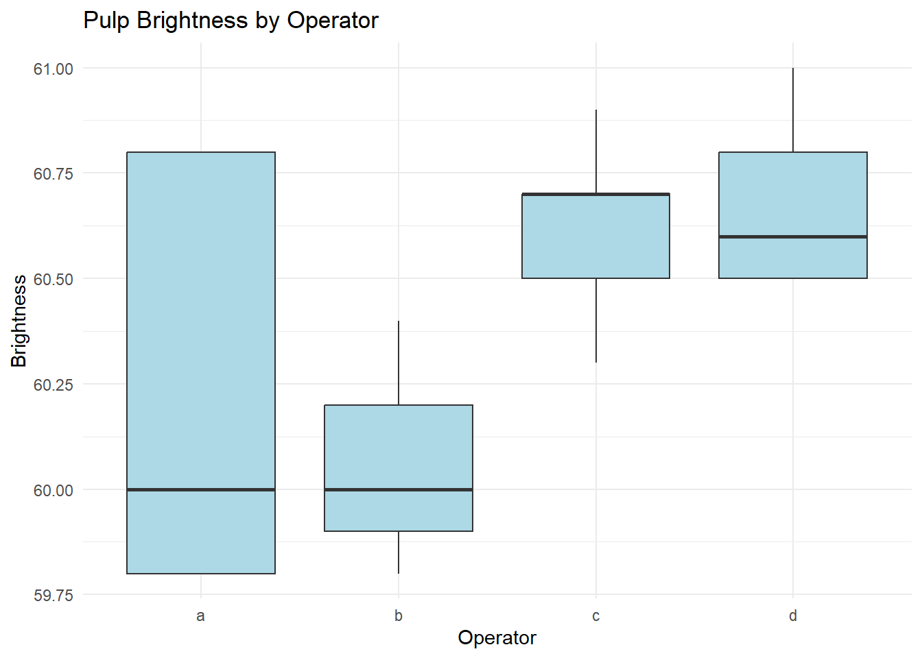
Figure 8.2: Pulp Brightness by Operator
8.8.1.3 Fitting the Mixed Model with lme4
library(lme4)

# Random intercepts model: operator as a random effect
mixed_model <- lmer(bright ~ 1 + (1 | operator), data = pulp)

# Model summary
summary(mixed_model)
#> Linear mixed model fit by REML. t-tests use Satterthwaite's method [
#> lmerModLmerTest]
#> Formula: bright ~ 1 + (1 | operator)
#>    Data: pulp
#>
#> REML criterion at convergence: 18.6
#>
#> Scaled residuals:
#>     Min      1Q  Median      3Q     Max
#> -1.4666 -0.7595 -0.1244  0.6281  1.6012
#>
#> Random effects:
#>  Groups   Name        Variance Std.Dev.
#>  operator (Intercept) 0.06808  0.2609
#>  Residual             0.10625  0.3260
#> Number of obs: 20, groups:  operator, 4
#>
#> Fixed effects:
#>             Estimate Std. Error      df t value Pr(>|t|)
#> (Intercept)  60.4000     0.1494  3.0000   404.2 3.34e-08 ***
#> ---
#> Signif. codes:  0 '***' 0.001 '**' 0.01 '*' 0.05 '.' 0.1 ' ' 1

# Fixed effects (overall mean)
fixef(mixed_model)
#> (Intercept)
#>        60.4

# Random effects (BLUPs)
ranef(mixed_model)
#> $operator
#>   (Intercept)
#> a  -0.1219403
#> b  -0.2591231
#> c   0.1676679
#> d   0.2133955
#>
#> with conditional variances for "operator"

# Variance components
VarCorr(mixed_model)
#>  Groups   Name        Std.Dev.
#>  operator (Intercept) 0.26093
#>  Residual             0.32596
re_dat <- as.data.frame(VarCorr(mixed_model))

# Intraclass Correlation Coefficient
rho <- re_dat[1, 'vcov'] / (re_dat[1, 'vcov'] + re_dat[2, 'vcov'])
rho
#> [1] 0.3905354
8.8.1.4 Inference with lmerTest
To obtain p-values for fixed effects using Satterthwaite’s approximation:
library(lmerTest)

# Model with p-values
summary(lmer(bright ~ 1 + (1 | operator), data = pulp))$coefficients
#>             Estimate Std. Error df  t value     Pr(>|t|)
#> (Intercept)     60.4  0.1494434  3 404.1664 3.340265e-08

# Confidence interval for the fixed effect
confint(mixed_model)[3,]
#>   2.5 %  97.5 %
#> 60.0713 60.7287
In this example, we can see that the confidence interval computed by confint from the lme4 package is very close to the one computed by confint from the lmerTest package.
8.8.1.5 Bayesian Mixed Model with MCMCglmm
library(MCMCglmm)

# Bayesian mixed model
mixed_model_bayes <- MCMCglmm(
  bright ~ 1,
  random = ~ operator,
  data = pulp,
  verbose = FALSE
)

# Posterior summaries
summary(mixed_model_bayes)$solutions
#>             post.mean l-95% CI u-95% CI eff.samp pMCMC
#> (Intercept)  60.40789  60.1488 60.69595     1000 0.001
Bayesian credible intervals may differ slightly from frequentist confidence intervals due to prior assumptions.
8.8.1.6 Predictions
# Random effects predictions (BLUPs)
ranef(mixed_model)$operator
#>   (Intercept)
#> a  -0.1219403
#> b  -0.2591231
#> c   0.1676679
#> d   0.2133955

# Predictions per operator
fixef(mixed_model) + ranef(mixed_model)$operator
#>   (Intercept)
#> a    60.27806
#> b    60.14088
#> c    60.56767
#> d    60.61340

# Equivalent using predict()
predict(mixed_model,
        newdata = data.frame(operator = c('a', 'b', 'c', 'd')))
#>        1        2        3        4
#> 60.27806 60.14088 60.56767 60.61340
For bootstrap confidence intervals, use:
bootMer(mixed_model, FUN = fixef, nsim = 100)
#>
#> PARAMETRIC BOOTSTRAP
#>
#>
#> Call:
#> bootMer(x = mixed_model, FUN = fixef, nsim = 100)
#>
#>
#> Bootstrap Statistics :
#>     original        bias    std. error
#> t1*     60.4 -0.0005452538    0.156374
8.8.2 Example 2: Penicillin Yield (GLMM with Blocking)
# Visualize yield by treatment and blend
ggplot(penicillin, aes(
  y = yield,
  x = treat,
  shape = blend,
  color = blend
)) +
  geom_point(size = 3) +
  labs(title = "Penicillin Yield by Treatment and Blend") +
  theme_minimal()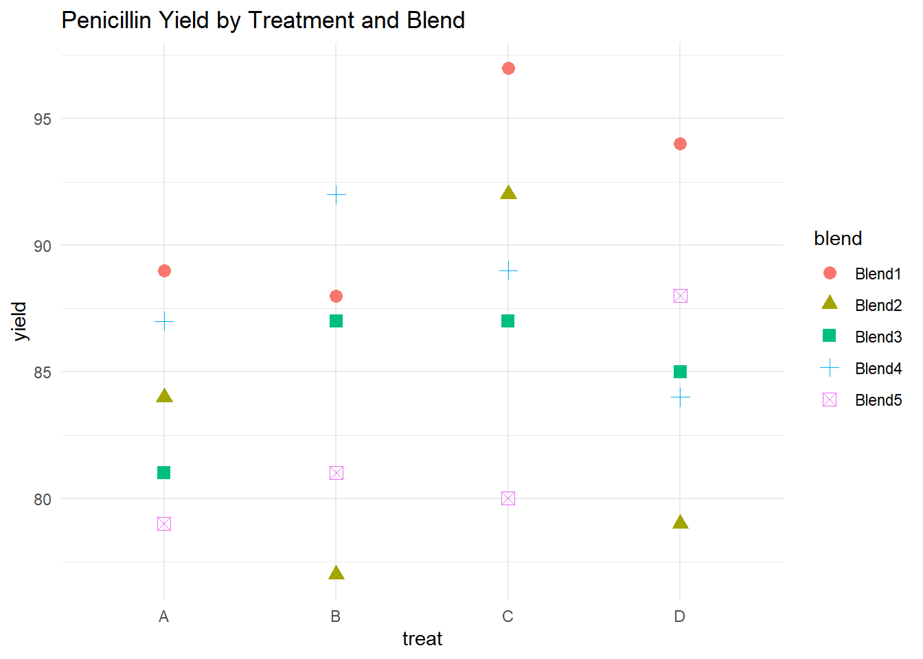
Figure 8.3: Penicillin Yield by Treatment and Blend
# Mixed model: blend as random effect, treatment as fixed
mixed_model <- lmer(yield ~ treat + (1 | blend), data = penicillin)
summary(mixed_model)
#> Linear mixed model fit by REML. t-tests use Satterthwaite's method [
#> lmerModLmerTest]
#> Formula: yield ~ treat + (1 | blend)
#>    Data: penicillin
#>
#> REML criterion at convergence: 103.8
#>
#> Scaled residuals:
#>     Min      1Q  Median      3Q     Max
#> -1.4152 -0.5017 -0.1644  0.6830  1.2836
#>
#> Random effects:
#>  Groups   Name        Variance Std.Dev.
#>  blend    (Intercept) 11.79    3.434
#>  Residual             18.83    4.340
#> Number of obs: 20, groups:  blend, 5
#>
#> Fixed effects:
#>             Estimate Std. Error     df t value Pr(>|t|)
#> (Intercept)   84.000      2.475 11.075  33.941 1.51e-12 ***
#> treatB         1.000      2.745 12.000   0.364   0.7219
#> treatC         5.000      2.745 12.000   1.822   0.0935 .
#> treatD         2.000      2.745 12.000   0.729   0.4802
#> ---
#> Signif. codes:  0 '***' 0.001 '**' 0.01 '*' 0.05 '.' 0.1 ' ' 1
#>
#> Correlation of Fixed Effects:
#>        (Intr) treatB treatC
#> treatB -0.555
#> treatC -0.555  0.500
#> treatD -0.555  0.500  0.500

# BLUPs for each blend
ranef(mixed_model)$blend
#>        (Intercept)
#> Blend1   4.2878788
#> Blend2  -2.1439394
#> Blend3  -0.7146465
#> Blend4   1.4292929
#> Blend5  -2.8585859
Testing for Treatment Effect
# ANOVA for fixed effects
anova(mixed_model)
#> Type III Analysis of Variance Table with Satterthwaite's method
#>       Sum Sq Mean Sq NumDF DenDF F value Pr(>F)
#> treat     70  23.333     3    12  1.2389 0.3387
Since the \(p\)-value \(> .05\), we fail to reject the null hypothesis (no treatment effect).
Model Comparison with Kenward-Roger Approximation
library(pbkrtest)

# Full model vs. null model
full_model <-
    lmer(yield ~ treat + (1 | blend), penicillin, REML = FALSE)
null_model <-
    lmer(yield ~ 1 + (1 | blend), penicillin, REML = FALSE)

# Kenward-Roger approximation
KRmodcomp(full_model, null_model)
#> large : yield ~ treat + (1 | blend)
#> small : yield ~ 1 + (1 | blend)
#>          stat     ndf     ddf F.scaling p.value
#> Ftest  1.2389  3.0000 12.0000         1  0.3387
The results are consistent with the earlier ANOVA: no significant treatment effect.
8.8.3 Example 3: Growth in Rats Over Time
rats <- read.csv(
    "images/rats.dat",
    header = FALSE,
    sep = ' ',
    col.names = c('Treatment', 'rat', 'age', 'y')
)

# Log-transformed time variable
rats$t <- log(1 + (rats$age - 45) / 10)
Model Fitting
# Treatment as fixed effect, random intercepts for rats
rat_model <- lmer(y ~ t:Treatment + (1 | rat), data = rats)
summary(rat_model)
#> Linear mixed model fit by REML. t-tests use Satterthwaite's method [
#> lmerModLmerTest]
#> Formula: y ~ t:Treatment + (1 | rat)
#>    Data: rats
#>
#> REML criterion at convergence: 932.4
#>
#> Scaled residuals:
#>      Min       1Q   Median       3Q      Max
#> -2.25574 -0.65898 -0.01163  0.58356  2.88309
#>
#> Random effects:
#>  Groups   Name        Variance Std.Dev.
#>  rat      (Intercept) 3.565    1.888
#>  Residual             1.445    1.202
#> Number of obs: 252, groups:  rat, 50
#>
#> Fixed effects:
#>                Estimate Std. Error       df t value Pr(>|t|)
#> (Intercept)     68.6074     0.3312  89.0275  207.13   <2e-16 ***
#> t:Treatmentcon   7.3138     0.2808 247.2762   26.05   <2e-16 ***
#> t:Treatmenthig   6.8711     0.2276 247.7097   30.19   <2e-16 ***
#> t:Treatmentlow   7.5069     0.2252 247.5196   33.34   <2e-16 ***
#> ---
#> Signif. codes:  0 '***' 0.001 '**' 0.01 '*' 0.05 '.' 0.1 ' ' 1
#>
#> Correlation of Fixed Effects:
#>             (Intr) t:Trtmntc t:Trtmnth
#> t:Tretmntcn -0.327
#> t:Tretmnthg -0.340  0.111
#> t:Tretmntlw -0.351  0.115     0.119
anova(rat_model)
#> Type III Analysis of Variance Table with Satterthwaite's method
#>             Sum Sq Mean Sq NumDF  DenDF F value    Pr(>F)
#> t:Treatment 3181.9  1060.6     3 223.21  734.11 < 2.2e-16 ***
#> ---
#> Signif. codes:  0 '***' 0.001 '**' 0.01 '*' 0.05 '.' 0.1 ' ' 1
Since the p-value is significant, we conclude that the treatment effect varies over time.
8.8.4 Example 4: Tree Water Use (Agridat)
# Visualizing water use by species and age
useOuterStrips(
  xyplot(water ~ day | species * age,
         dat, group = tree,
         type = c('p', 'smooth'),
         main = "harris.wateruse 2 species, 2 ages (10 trees each)",
         as.table = TRUE)
)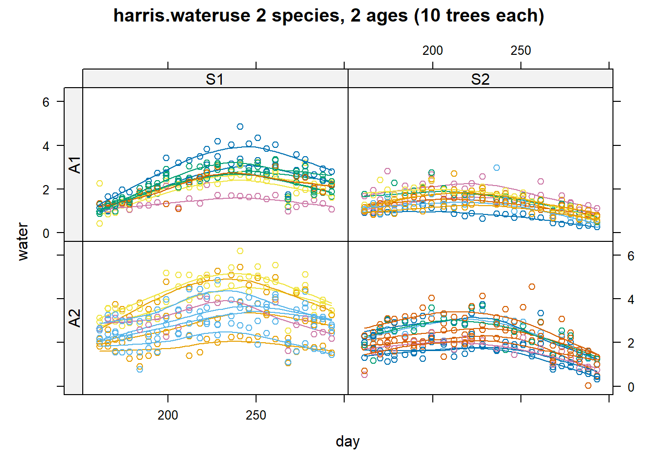
Figure 8.4: Species by Age
Remove outlier
Plot between water use and day for one age and species group
xyplot(
    water ~ day | tree,
    dat,
    subset   = age == "A2" & species == "S2",
    as.table = TRUE,
    type     = c('p', 'smooth'),
    ylab     = "Water use profiles of individual trees",
    main     = "harris.wateruse (Age 2, Species 2)"
)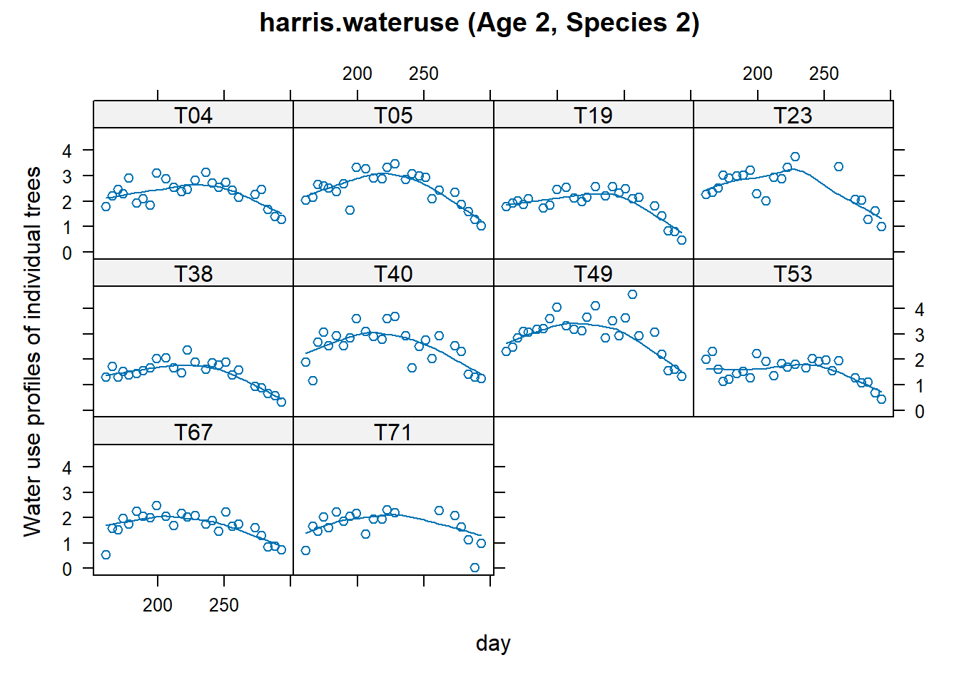
Figure 8.5: harris.wateruse (Age 2, Species 2)
# Rescale day for nicer output, and convergence issues
dat <- transform(dat, ti = day / 100)
# add quadratic term
dat <- transform(dat, ti2 = ti * ti)

# Start with a subgroup: age 2, species 2
d22 <- droplevels(subset(dat, age == "A2" & species == "S2"))
Fitting with nlme using lme
library(nlme)

## We use pdDiag() to get uncorrelated random effects
m1n <- lme(
    water ~ 1 + ti + ti2,
    #intercept, time and time-squared = fixed effects
    data = d22,
    na.action = na.omit,
    random = list(tree = pdDiag(~ 1 + ti + ti2))
    # random intercept, time
    # and time squared per tree = random effects
)

# for all trees
# m1n <- lme(
#   water ~ 1 + ti + ti2,
#   random = list(tree = pdDiag(~ 1 + ti + ti2)),
#   data = dat,
#   na.action = na.omit
# )

summary(m1n)
#> Linear mixed-effects model fit by REML
#>   Data: d22
#>        AIC     BIC    logLik
#>   276.5142 300.761 -131.2571
#>
#> Random effects:
#>  Formula: ~1 + ti + ti2 | tree
#>  Structure: Diagonal
#>         (Intercept)           ti          ti2  Residual
#> StdDev:   0.5187869 1.631223e-05 4.374982e-06 0.3836614
#>
#> Fixed effects:  water ~ 1 + ti + ti2
#>                  Value Std.Error  DF   t-value p-value
#> (Intercept) -10.798799 0.8814666 227 -12.25094       0
#> ti           12.346704 0.7827112 227  15.77428       0
#> ti2          -2.838503 0.1720614 227 -16.49704       0
#>  Correlation:
#>     (Intr) ti
#> ti  -0.979
#> ti2  0.970 -0.997
#>
#> Standardized Within-Group Residuals:
#>         Min          Q1         Med          Q3         Max
#> -3.07588246 -0.58531056  0.01210209  0.65402695  3.88777402
#>
#> Number of Observations: 239
#> Number of Groups: 10

ranef(m1n)
#>     (Intercept)            ti           ti2
#> T04   0.1985796  2.070606e-09  6.397103e-10
#> T05   0.3492827  3.199664e-10 -6.211457e-11
#> T19  -0.1978989 -9.879555e-10 -2.514502e-10
#> T23   0.4519003 -4.206418e-10 -3.094113e-10
#> T38  -0.6457494 -2.069198e-09 -4.227912e-10
#> T40   0.3739432  4.199061e-10 -3.260161e-11
#> T49   0.8620648  1.160387e-09 -6.925457e-12
#> T53  -0.5655049 -1.064849e-09 -5.870462e-11
#> T67  -0.4394623 -4.482549e-10  2.752922e-11
#> T71  -0.3871552  1.020034e-09  4.767595e-10

fixef(m1n)
#> (Intercept)          ti         ti2
#>  -10.798799   12.346704   -2.838503
Fitting with lme4 using lmer
library(lme4)

m1lmer <-
    lmer(water ~ 1 + ti + ti2 + (ti + ti2 ||
                                     tree),
         data = d22,
         na.action = na.omit)

# for all trees
# m1lmer <- lmer(water ~ 1 + ti + ti2 + (ti + ti2 || tree),
#                data = dat, na.action = na.omit)

# summary(m1lmer)
ranef(m1lmer)
#> $tree
#>     (Intercept) ti ti2
#> T04   0.1985796  0   0
#> T05   0.3492827  0   0
#> T19  -0.1978989  0   0
#> T23   0.4519003  0   0
#> T38  -0.6457494  0   0
#> T40   0.3739432  0   0
#> T49   0.8620648  0   0
#> T53  -0.5655049  0   0
#> T67  -0.4394623  0   0
#> T71  -0.3871552  0   0
#>
#> with conditional variances for "tree"

fixef(m1lmer)
#> (Intercept)          ti         ti2
#>  -10.798799   12.346704   -2.838503
Notes:
||double pipes = uncorrelated random effects- To remove the intercept term:
(0+ti|tree)(ti-1|tree)
m1l <-
    lmer(water ~ 1 + ti + ti2
         + (1 | tree) + (0 + ti | tree)
         + (0 + ti2 | tree), data = d22)
ranef(m1l)
#> $tree
#>     (Intercept) ti ti2
#> T04   0.1985796  0   0
#> T05   0.3492827  0   0
#> T19  -0.1978989  0   0
#> T23   0.4519003  0   0
#> T38  -0.6457494  0   0
#> T40   0.3739432  0   0
#> T49   0.8620648  0   0
#> T53  -0.5655049  0   0
#> T67  -0.4394623  0   0
#> T71  -0.3871552  0   0
#>
#> with conditional variances for "tree"
fixef(m1l)
#> (Intercept)          ti         ti2
#>  -10.798799   12.346704   -2.838503
Adding Correlation Structure
m2n <- lme(
    water ~ 1 + ti + ti2,
    data = d22,
    random = ~ 1 | tree,
    cor = corExp(form =  ~ day | tree),
    na.action = na.omit
)

# for all trees
# m2n <- lme(
#   water ~ 1 + ti + ti2,
#   random = ~ 1 | tree,
#   cor = corExp(form = ~ day | tree),
#   data = dat,
#   na.action = na.omit
# )

summary(m2n)
#> Linear mixed-effects model fit by REML
#>   Data: d22
#>        AIC      BIC   logLik
#>   263.3081 284.0911 -125.654
#>
#> Random effects:
#>  Formula: ~1 | tree
#>         (Intercept)  Residual
#> StdDev:   0.5154042 0.3925777
#>
#> Correlation Structure: Exponential spatial correlation
#>  Formula: ~day | tree
#>  Parameter estimate(s):
#>    range
#> 3.794624
#> Fixed effects:  water ~ 1 + ti + ti2
#>                  Value Std.Error  DF   t-value p-value
#> (Intercept) -11.223310 1.0988725 227 -10.21348       0
#> ti           12.712094 0.9794235 227  12.97916       0
#> ti2          -2.913682 0.2148551 227 -13.56115       0
#>  Correlation:
#>     (Intr) ti
#> ti  -0.985
#> ti2  0.976 -0.997
#>
#> Standardized Within-Group Residuals:
#>         Min          Q1         Med          Q3         Max
#> -3.04861039 -0.55703950  0.00278101  0.62558762  3.80676991
#>
#> Number of Observations: 239
#> Number of Groups: 10
ranef(m2n)
#>     (Intercept)
#> T04   0.1929971
#> T05   0.3424631
#> T19  -0.1988495
#> T23   0.4538660
#> T38  -0.6413664
#> T40   0.3769378
#> T49   0.8410043
#> T53  -0.5528236
#> T67  -0.4452930
#> T71  -0.3689358
fixef(m2n)
#> (Intercept)          ti         ti2
#>  -11.223310   12.712094   -2.913682
Key Takeaways
lme4is preferred for general mixed models due to efficiency and simplicity.nlmeis powerful for complex correlation structures and nested designs.Bayesian models (e.g.,
MCMCglmm) offer flexible inference under uncertainty.Always consider model diagnostics and random effects structure carefully.