17.7 Packages for Marginal Effects
Several R packages compute marginal effects for regression models, each with different features and functionalities. The primary packages include:
marginaleffects– A modern, flexible, and efficient package.margins– A widely used package for replicating Stata’smarginscommand.mfx– A package tailored for Generalized Linear Models (glm).
These tools help analyze how small changes in explanatory variables impact the dependent variable.
17.7.1 marginaleffects Package (Recommended)
The marginaleffects package is the successor to margins and emtrends, offering a faster, more efficient, and more flexible approach to estimating marginal effects.
Why Use marginaleffects?
Supports interaction effects and complex models
Computes marginal effects, marginal means, and counterfactuals
Integrates well with ggplot2 for visualization
Works with many model types (linear, logistic, Poisson, etc.)
Limitation:
- No built-in function for multiple comparisons correction, but you can use
p.adjust()for adjustment.
Key Definitions
- Marginal Effects: The partial derivative (slope) of the outcome with respect to each variable.
marginspackage defines marginal effects as “partial derivatives of the regression equation with respect to each variable in the model for each unit in the data.”
- Marginal Means: The expected outcome averaged over a grid of predictor values.
Computing Predictions and Marginal Effects
library(marginaleffects)
library(tidyverse)
data(mtcars)


# Fit a regression model with interaction terms
mod <- lm(mpg ~ hp * wt * am, data = mtcars)

# Get predicted values
predictions(mod) %>% head()
#>
#>  Estimate Std. Error    z Pr(>|z|)     S 2.5 % 97.5 %
#>      22.5      0.884 25.4   <0.001 471.7  20.8   24.2
#>      20.8      1.194 17.4   <0.001 223.3  18.5   23.1
#>      25.3      0.709 35.7   <0.001 922.7  23.9   26.7
#>      20.3      0.704 28.8   <0.001 601.5  18.9   21.6
#>      17.0      0.712 23.9   <0.001 416.2  15.6   18.4
#>      19.7      0.875 22.5   <0.001 368.8  17.9   21.4
#>
#> Type: response

# Create a reference grid for prediction
newdata <- datagrid(am = 0,
                    wt = c(2, 4),
                    model = mod)
# Plot predictions for 'hp' and 'wt'
marginaleffects::plot_predictions(mod,
newdata = newdata,
condition = c("hp", "wt"))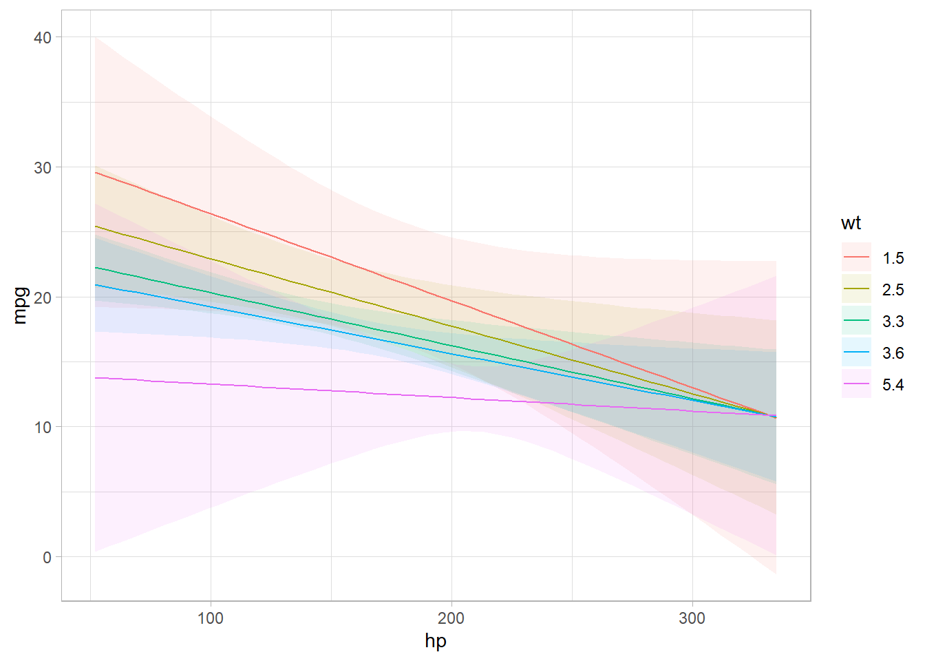
Figure 17.2: Line Chart Coefficients
Computing Marginal Effects
# Compute Average Marginal Effects (AME)
mfx <- marginaleffects::slopes(mod, variables = c("hp", "wt"))
head(mfx)
#>
#>  Estimate Std. Error     z Pr(>|z|)   S   2.5 %    97.5 %
#>   -0.0369     0.0185 -2.00  0.04598 4.4 -0.0732 -0.000659
#>   -0.0287     0.0156 -1.84  0.06630 3.9 -0.0593  0.001931
#>   -0.0466     0.0226 -2.06  0.03945 4.7 -0.0909 -0.002249
#>   -0.0423     0.0133 -3.18  0.00146 9.4 -0.0683 -0.016232
#>   -0.0390     0.0134 -2.91  0.00363 8.1 -0.0653 -0.012730
#>   -0.0387     0.0135 -2.87  0.00409 7.9 -0.0652 -0.012289
#>
#> Term: hp
#> Type: response
#> Comparison: dY/dX

# Compute Group-Average Marginal Effects
head(marginaleffects::slopes(mod, by = "hp", variables = "am"))
#>
#>  hp Estimate Std. Error      z Pr(>|z|)   S 2.5 % 97.5 %
#>  52     3.98       5.20  0.764    0.445 1.2 -6.22  14.18
#>  62    -2.77       2.51 -1.107    0.268 1.9 -7.68   2.14
#>  65     3.00       4.13  0.725    0.468 1.1 -5.10  11.10
#>  66     2.03       3.48  0.582    0.561 0.8 -4.80   8.85
#>  91     1.86       2.76  0.674    0.500 1.0 -3.54   7.26
#>  93     1.20       2.35  0.511    0.609 0.7 -3.40   5.80
#>
#> Term: am
#> Type: response
#> Comparison: 1 - 0

# Marginal Effects at Representative Values (MER)
marginaleffects::slopes(mod, newdata = datagrid(am = 0, wt = c(2, 4)))
#>
#>  Term Contrast am wt Estimate Std. Error      z Pr(>|z|)   S   2.5 %   97.5 %
#>    am    1 - 0  0  2   2.5474     2.7891  0.913   0.3611 1.5 -2.9191  8.01403
#>    am    1 - 0  0  4  -2.9541     3.0348 -0.973   0.3304 1.6 -8.9021  2.99400
#>    hp    dY/dX  0  2  -0.0598     0.0283 -2.115   0.0344 4.9 -0.1153 -0.00439
#>    hp    dY/dX  0  4  -0.0309     0.0187 -1.654   0.0982 3.3 -0.0676  0.00573
#>    wt    dY/dX  0  2  -2.6716     1.4149 -1.888   0.0590 4.1 -5.4449  0.10159
#>    wt    dY/dX  0  4  -2.6716     1.4154 -1.888   0.0591 4.1 -5.4458  0.10248
#>
#> Type: response

# Marginal Effects at the Mean (MEM)
marginaleffects::slopes(mod, newdata = "mean")
#>
#>  Term Contrast Estimate Std. Error      z Pr(>|z|)   S   2.5 %  97.5 %
#>    am    1 - 0  -0.8009     1.5219 -0.526  0.59871 0.7 -3.7837  2.1819
#>    hp    dY/dX  -0.0422     0.0133 -3.181  0.00147 9.4 -0.0683 -0.0162
#>    wt    dY/dX  -2.6716     1.4151 -1.888  0.05903 4.1 -5.4452  0.1019
#>
#> Type: response
Counterfactual Comparisons
# Counterfactual comparison: Effect of changing 'am' from 0 to 1
comparisons(mod, variables = list(am = 0:1))
#>
#>  Estimate Std. Error      z Pr(>|z|)   S 2.5 % 97.5 %
#>     0.325       1.68  0.193    0.847 0.2 -2.97   3.62
#>    -0.544       1.57 -0.347    0.729 0.5 -3.62   2.53
#>     1.201       2.35  0.511    0.609 0.7 -3.40   5.80
#>    -1.703       1.87 -0.912    0.362 1.5 -5.36   1.96
#>    -0.615       1.68 -0.366    0.715 0.5 -3.91   2.68
#> --- 22 rows omitted. See ?print.marginaleffects ---
#>     4.081       3.94  1.037    0.300 1.7 -3.63  11.79
#>     2.106       2.29  0.920    0.358 1.5 -2.38   6.59
#>     0.895       1.64  0.544    0.586 0.8 -2.33   4.12
#>     4.027       3.24  1.243    0.214 2.2 -2.32  10.38
#>    -0.237       1.59 -0.149    0.881 0.2 -3.35   2.87
#> Term: am
#> Type: response
#> Comparison: 1 - 0
17.7.2 margins Package
The margins package is a popular choice, designed to replicate Stata’s margins command in R. It provides marginal effects for each variable in a model, including interaction terms. margins define:
- Average Partial Effects: The contribution of each variable to the outcome scale, conditional on the other variables involved in the link function transformation of the linear predictor.
- Average Marginal Effects: The marginal contribution of each variable on the scale of the linear predictor.
- Average marginal effects represent the mean of these unit-specific partial derivatives over a given sample.
Key Features
Computes Average Partial Effects (APE).
Supports Marginal Effects at the Mean (MEM).
Provides visualizations of marginal effects.
Limitation:
- Slower than
marginaleffects, especially with large datasets.
library(margins)

# Fit a linear model with interactions
mod <- lm(mpg ~ cyl * hp + wt, data = mtcars)

# Compute marginal effects
summary(margins(mod))
#>  factor     AME     SE       z      p   lower   upper
#>     cyl  0.0381 0.5999  0.0636 0.9493 -1.1376  1.2139
#>      hp -0.0463 0.0145 -3.1909 0.0014 -0.0748 -0.0179
#>      wt -3.1198 0.6613 -4.7175 0.0000 -4.4160 -1.8236

# Equivalent function for summary
margins_summary(mod)
#>  factor     AME     SE       z      p   lower   upper
#>     cyl  0.0381 0.5999  0.0636 0.9493 -1.1376  1.2139
#>      hp -0.0463 0.0145 -3.1909 0.0014 -0.0748 -0.0179
#>      wt -3.1198 0.6613 -4.7175 0.0000 -4.4160 -1.8236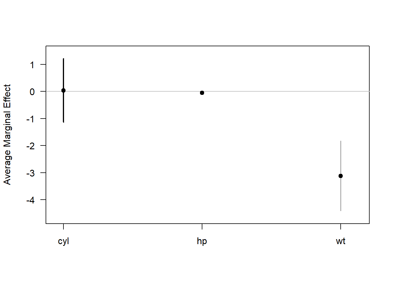
Figure 17.3: Average Marginal Effect
Marginal Effects at Representative Values
# Compute marginal effects when 'hp' = 150
margins(mod, at = list(hp = 150)) %>% summary()
#>  factor       hp     AME     SE       z      p   lower   upper
#>     cyl 150.0000  0.1009 0.6128  0.1647 0.8692 -1.1001  1.3019
#>      hp 150.0000 -0.0463 0.0145 -3.1909 0.0014 -0.0748 -0.0179
#>      wt 150.0000 -3.1198 0.6613 -4.7175 0.0000 -4.4160 -1.8236
17.7.3 mfx Package
The mfx package is specialized for GLMs, computing marginal effects for probit, logit, Poisson, and other count models.
Limitation:
- Computes only marginal effects for each variable, not the average marginal effect.
Supported Models in mfx
| Model | Outcome Type | Function |
|---|---|---|
| Probit | Binary | probitmfx() |
| Logit | Binary | logitmfx() |
| Poisson | Count | poissonmfx() |
| Negative Binomial | Count | negbinmfx() |
| Beta | Rate | betamfx() |
Example: Poisson Regression
library(mfx)
data("mtcars")

# Fit a Poisson model and compute marginal effects
poissonmfx(formula = vs ~ mpg * cyl * disp, data = mtcars)
#> Call:
#> poissonmfx(formula = vs ~ mpg * cyl * disp, data = mtcars)
#>
#> Marginal Effects:
#>                    dF/dx   Std. Err.       z  P>|z|
#> mpg           1.4722e-03  8.7531e-03  0.1682 0.8664
#> cyl           6.6420e-03  3.9263e-02  0.1692 0.8657
#> disp          1.5899e-04  9.4555e-04  0.1681 0.8665
#> mpg:cyl      -3.4698e-04  2.0564e-03 -0.1687 0.8660
#> mpg:disp     -7.6794e-06  4.5545e-05 -0.1686 0.8661
#> cyl:disp     -3.3837e-05  1.9919e-04 -0.1699 0.8651
#> mpg:cyl:disp  1.6812e-06  9.8919e-06  0.1700 0.8650
For more details, see the mfx vignette.
17.7.4 Comparison of Packages
| Feature | marginaleffects (Recommended) |
margins |
mfx |
|---|---|---|---|
| Computes AME | Yes | Yes | No |
| Computes MEM | Yes | Yes | No |
| Computes MER | Yes | Yes | No |
| Supports GLM Models | Yes | Yes | Yes (but limited to glm) |
| Works with Interactions | Yes | Yes | No |
| Fast and Efficient | Yes | No (slower) | Yes (for GLMs) |
| Supports Counterfactuals | Yes | No | No |