33.8 Confounders in Event Studies
A major challenge in event studies is controlling for confounding events, which could bias the estimation of abnormal returns.
33.8.1 Types of Confounding Events
(McWilliams and Siegel 1997) suggest excluding firms that experience other major events within a two-day window around the focal event. These include:
- Financial announcements: Earnings reports, stock buybacks, dividend changes, IPOs.
- Corporate actions: Mergers, acquisitions, spin-offs, stock splits, debt defaults.
- Executive changes: CEO/CFO resignations or appointments.
- Operational changes: Layoffs, restructurings, lawsuits, joint ventures.
Fornell et al. (2006) recommend:
- One-day event period: The date when Wall Street Journal publishes the ACSI announcement.
- Five-day window (before and after the event) to rule out other news (from PR Newswires, Dow Jones, Business Wires).
Events controlled for include:
M&A, spin-offs, stock splits.
CEO or CFO changes.
Layoffs, restructurings, lawsuits.
A useful data source for identifying confounding events is Capital IQ’s Key Developments, which captures almost all important corporate events.
33.8.2 Should We Exclude Confounded Observations?
A. Sorescu, Warren, and Ertekin (2017) investigated confounding events in short-term event windows using:
RavenPack dataset (2000-2013).
3-day event windows for 3,982 US publicly traded firms.
Key Findings:
- The difference between the full sample and the sample without confounded events was statistically insignificant.
- Conclusion: Excluding confounded observations may not be necessary in short-term event studies.
Why?
- Selection bias risk: Researchers may selectively exclude events, introducing bias.
- Increasing exclusions over time: As time progresses, more events need to be excluded, reducing statistical power.
- Short-term windows minimize confounder effects.
33.8.3 Simulation Study: Should We Exclude Correlated and Uncorrelated Events?
To illustrate the impact of correlated and uncorrelated events, let’s conduct a simulation study.
We consider three event types:
- Focal events (events of interest).
- Correlated events (events that often co-occur with focal events).
- Uncorrelated events (random events that might coincide with focal events).
We will analyze the impact of including vs. excluding correlated and uncorrelated events.
# Load required libraries
library(dplyr)
library(ggplot2)
library(tidyr)
library(tidyverse)

# Parameters
n                  <- 100000         # Number of observations
n_focal            <- round(n * 0.2) # Number of focal events
overlap_correlated <- 0.5            # Overlapping percentage between focal and correlated events

# Function to compute mean and confidence interval
mean_ci <- function(x) {
    m <- mean(x)
    ci <- qt(0.975, length(x)-1) * sd(x) / sqrt(length(x)) # 95% confidence interval
    list(mean = m, lower = m - ci, upper = m + ci)
}


# Simulate data
set.seed(42)
data <- tibble(
    date       = seq.Date(
        from = as.Date("2010-01-01"),
        by = "day",
        length.out = n
    ),
    # Date sequence
    focal      = rep(0, n),
    correlated = rep(0, n),
    ab_ret     = rnorm(n)
)


# Define focal events
focal_idx <- sample(1:n, n_focal)
data$focal[focal_idx] <- 1

true_effect <- 0.25

# Adjust the ab_ret for the focal events to have a mean of true_effect
data$ab_ret[focal_idx] <-
    data$ab_ret[focal_idx] - mean(data$ab_ret[focal_idx]) + true_effect


# Determine the number of correlated events that overlap with focal and those that don't
n_correlated_overlap <-
    round(length(focal_idx) * overlap_correlated)
n_correlated_non_overlap <- n_correlated_overlap

# Sample the overlapping correlated events from the focal indices
correlated_idx <- sample(focal_idx, size = n_correlated_overlap)

# Get the remaining indices that are not part of focal
remaining_idx <- setdiff(1:n, focal_idx)

# Check to ensure that we're not attempting to sample more than the available remaining indices
if (length(remaining_idx) < n_correlated_non_overlap) {
    stop("Not enough remaining indices for non-overlapping correlated events")
}

# Sample the non-overlapping correlated events from the remaining indices
correlated_non_focal_idx <-
    sample(remaining_idx, size = n_correlated_non_overlap)

# Combine the two to get all correlated indices
all_correlated_idx <- c(correlated_idx, correlated_non_focal_idx)

# Set the correlated events in the data
data$correlated[all_correlated_idx] <- 1


# Inflate the effect for correlated events to have a mean of
correlated_non_focal_idx <-
    setdiff(all_correlated_idx, focal_idx) # Fixing the selection of non-focal correlated events
data$ab_ret[correlated_non_focal_idx] <-
    data$ab_ret[correlated_non_focal_idx] - mean(data$ab_ret[correlated_non_focal_idx]) + 1


# Define the numbers of uncorrelated events for each scenario
num_uncorrelated <- c(5, 10, 20, 30, 40)

# Define uncorrelated events
for (num in num_uncorrelated) {
    for (i in 1:num) {
        data[paste0("uncorrelated_", i)] <- 0
        uncorrelated_idx <- sample(1:n, round(n * 0.1))
        data[uncorrelated_idx, paste0("uncorrelated_", i)] <- 1
    }
}


# Define uncorrelated columns and scenarios
unc_cols <- paste0("uncorrelated_", 1:num_uncorrelated)
results <- tibble(
    Scenario = c(
        "Include Correlated",
        "Correlated Effects",
        "Exclude Correlated",
        "Exclude Correlated and All Uncorrelated"
    ),
    MeanEffect = c(
        mean_ci(data$ab_ret[data$focal == 1])$mean,
        mean_ci(data$ab_ret[data$focal == 0 |
                                data$correlated == 1])$mean,
        mean_ci(data$ab_ret[data$focal == 1 &
                                data$correlated == 0])$mean,
        mean_ci(data$ab_ret[data$focal == 1 &
                                data$correlated == 0 &
                                rowSums(data[, paste0("uncorrelated_", 1:num_uncorrelated)]) == 0])$mean
    ),
    LowerCI = c(
        mean_ci(data$ab_ret[data$focal == 1])$lower,
        mean_ci(data$ab_ret[data$focal == 0 |
                                data$correlated == 1])$lower,
        mean_ci(data$ab_ret[data$focal == 1 &
                                data$correlated == 0])$lower,
        mean_ci(data$ab_ret[data$focal == 1 &
                                data$correlated == 0 &
                                rowSums(data[, paste0("uncorrelated_", 1:num_uncorrelated)]) == 0])$lower
    ),
    UpperCI = c(
        mean_ci(data$ab_ret[data$focal == 1])$upper,
        mean_ci(data$ab_ret[data$focal == 0 |
                                data$correlated == 1])$upper,
        mean_ci(data$ab_ret[data$focal == 1 &
                                data$correlated == 0])$upper,
        mean_ci(data$ab_ret[data$focal == 1 &
                                data$correlated == 0 &
                                rowSums(data[, paste0("uncorrelated_", 1:num_uncorrelated)]) == 0])$upper
    )
)

# Add the scenarios for excluding 5, 10, 20, and 50 uncorrelated
for (num in num_uncorrelated) {
    unc_cols <- paste0("uncorrelated_", 1:num)
    results <- results %>%
        add_row(
            Scenario = paste("Exclude", num, "Uncorrelated"),
            MeanEffect = mean_ci(data$ab_ret[data$focal == 1 &
                                                 data$correlated == 0 &
                                                 rowSums(data[, unc_cols]) == 0])$mean,
            LowerCI = mean_ci(data$ab_ret[data$focal == 1 &
                                              data$correlated == 0 &
                                              rowSums(data[, unc_cols]) == 0])$lower,
            UpperCI = mean_ci(data$ab_ret[data$focal == 1 &
                                              data$correlated == 0 &
                                              rowSums(data[, unc_cols]) == 0])$upper
        )
}


ggplot(results,
       aes(
           x = factor(Scenario, levels = Scenario),
           y = MeanEffect,
           ymin = LowerCI,
           ymax = UpperCI
       )) +
    geom_pointrange() +
    coord_flip() +
    ylab("Mean Effect") +
    xlab("Scenario") +
    ggtitle("Mean Effect of Focal Events under Different Scenarios") +
    geom_hline(yintercept = true_effect,
               linetype = "dashed",
color = "red") 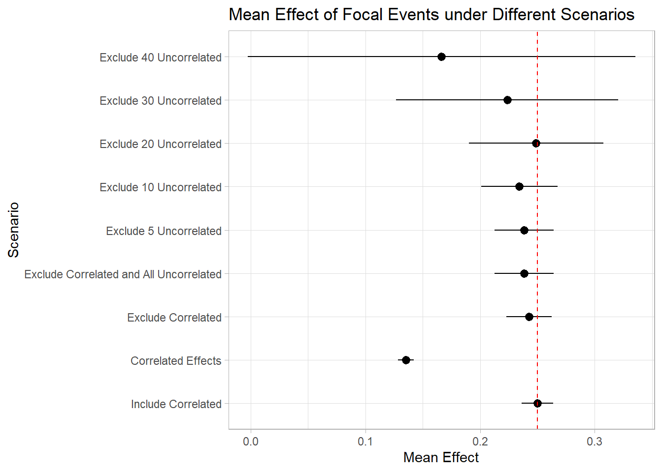
As depicted in the plot, the inclusion of correlated events demonstrates minimal impact on the estimation of our focal events. Conversely, excluding these correlated events can diminish our statistical power. This is true in cases of pronounced correlation.
However, the consequences of excluding unrelated events are notably more significant. It becomes evident that by omitting around 40 unrelated events from our study, we lose the ability to accurately identify the true effects of the focal events. In reality and within research, we often rely on the Key Developments database, excluding over 150 events, a practice that can substantially impair our capacity to ascertain the authentic impact of the focal events.
This little experiment really drives home the point – you better have a darn good reason to exclude an event from your study!