17.5 Comparison: Delta Method vs. Alternative Approaches
| Method | Description | Pros | Cons |
|---|---|---|---|
| Delta Method | Uses Taylor expansion to approximate variance | Computationally efficient | Accuracy depends on linearity assumption |
| Analytical Derivation | Directly derives probability function | Exact solution (if feasible) | Can be mathematically complex |
| Simulation/Bootstrapping | Uses repeated sampling from estimated distribution | No assumptions on functional form | Computationally expensive |
When to Use the Delta Method:
When you need a quick approximation for standard errors.
When the function \(G(\beta)\) is smooth and differentiable.
When working with large sample sizes, where asymptotic normality holds.
For deeper exploration, refer to these excellent resources:
Advanced: modmarg package documentation – covers implementation of the Delta Method in R.
Intermediate: UCLA Statistical Consulting – a practical FAQ on the Delta Method.
17.5.1 Example: Applying the Delta Method in a logistic regression
To illustrate, let’s apply the Delta Method to compute the standard error of a nonlinear transformation of regression coefficients.
In logistic regression, the estimated coefficient \(\hat{\beta}\) represents the log-odds change for a one-unit increase in \(X\). However, we often want the odds ratio, which is:
\[ G(\beta) = e^{\beta}. \]
By the Delta Method, the variance of \(e^{\beta}\) is:
\[ \text{Var}(e^{\beta}) \approx e^{2\beta} \cdot \text{Var}(\beta). \]
# Load necessary packages
library(ggplot2)
library(margins)
library(sandwich)
library(lmtest)

# Simulate data
set.seed(123)
n <- 100
X <- rnorm(n)  # Simulate independent variable
# Generate binary outcome using logistic model
Y <-
    rbinom(n, 1, plogis(0.5 + 0.8 * X))

# Logistic regression
logit_model <- glm(Y ~ X, family = binomial(link = "logit"))

# Extract coefficient and variance
beta_hat <- coef(logit_model)["X"]   # Estimated coefficient
var_beta_hat <- vcov(logit_model)["X", "X"]  # Variance of beta_hat

# Apply Delta Method
odds_ratio <- exp(beta_hat)  # Transform beta to odds ratio
se_odds_ratio <-
    sqrt(odds_ratio ^ 2 * var_beta_hat)  # Delta Method SE

# Compute 95% Confidence Interval
lower_CI <- exp(beta_hat - 1.96 * sqrt(var_beta_hat))
upper_CI <- exp(beta_hat + 1.96 * sqrt(var_beta_hat))

# Display results
results <- data.frame(
    Term = "X",
    Odds_Ratio = odds_ratio,
    SE = se_odds_ratio,
    Lower_CI = lower_CI,
    Upper_CI = upper_CI
)

print(results)
#>   Term Odds_Ratio        SE Lower_CI Upper_CI
#> X    X   2.655431 0.7677799 1.506669 4.680069

# ---- VISUALIZATION 1: Distribution of Simulated Odds Ratios ----
set.seed(123)
# Simulate beta estimates
simulated_betas <-
    rnorm(1000, mean = beta_hat, sd = sqrt(var_beta_hat))
simulated_odds_ratios <-
exp(simulated_betas) # Apply transformationggplot(data.frame(Odds_Ratio = simulated_odds_ratios),
aes(x = Odds_Ratio)) +
geom_histogram(
color = "black",
fill = "skyblue",
bins = 50,
alpha = 0.7
) +
geom_vline(
xintercept = odds_ratio,
color = "red",
linetype = "dashed",
linewidth = 1.2
) +
geom_vline(
xintercept = lower_CI,
color = "blue",
linetype = "dotted",
linewidth = 1.2
) +
geom_vline(
xintercept = upper_CI,
color = "blue",
linetype = "dotted",
linewidth = 1.2
) +
labs(title = "Distribution of Simulated Odds Ratios",
x = "Odds Ratio",
y = "Frequency") +
theme_minimal()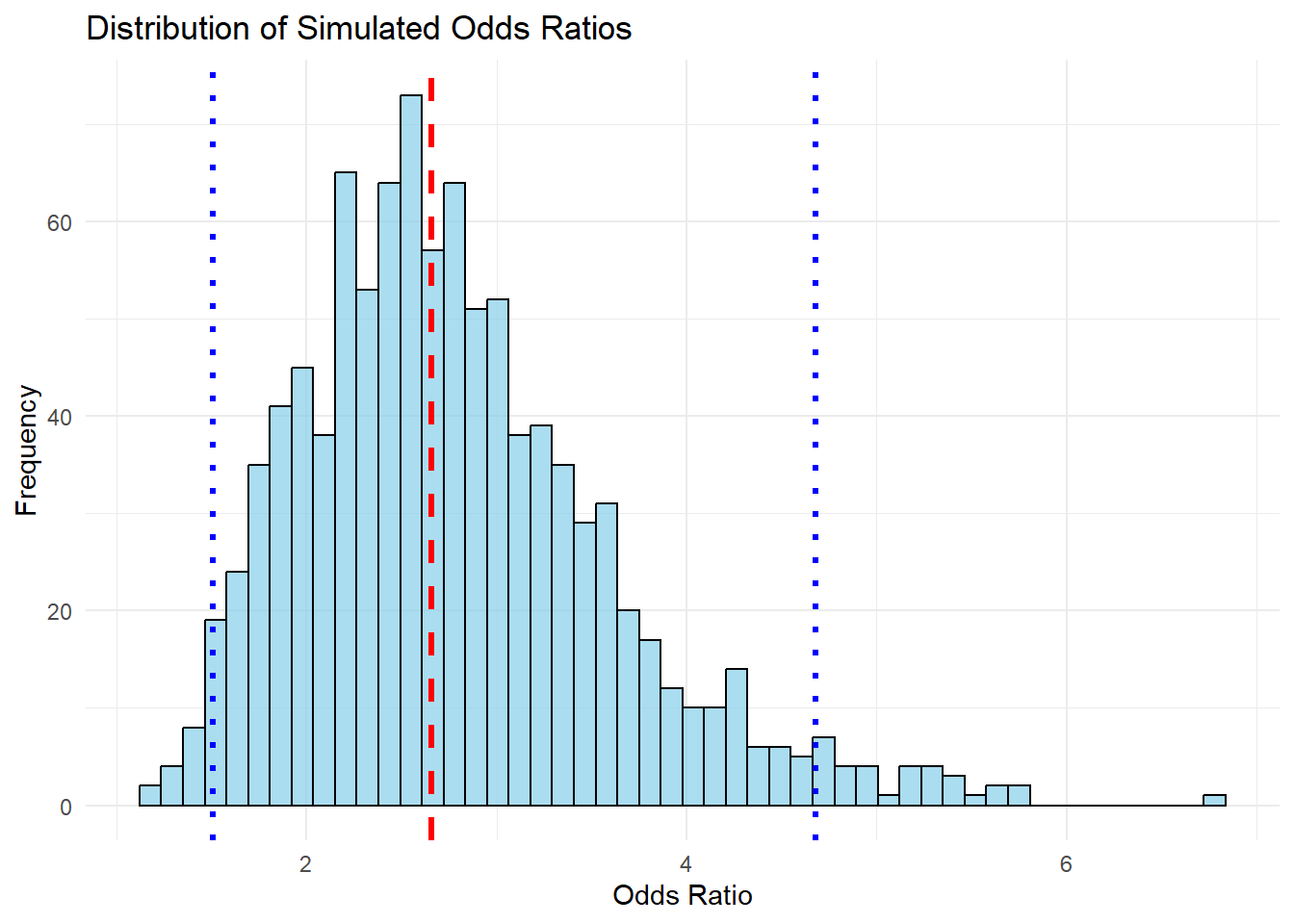
Figure 17.1: Distribution of Simulated Odds Ratios
Odds Ratio Computation
The odds ratio is the exponentiated coefficient \(e^{\hat{\beta}}\), which represents the multiplicative change in the odds of \(Y = 1\) for a one-unit increase in \(X\).
If \(\hat{\beta} = 0.8\), then \(e^{0.8} \approx 2.23\), meaning a one-unit increase in \(X\) increases the odds of \(Y = 1\) by 123%.
Standard Error via Delta Method
Since \(\beta\) follows a normal distribution, its transformation \(e^\beta\) is not normally distributed but rather follows a log-normal shape.
The Delta Method approximates the standard error of \(e^\beta\) using: \[ SE(e^\beta) = \sqrt{e^{2\beta} \cdot \text{Var}(\beta)} \]
Confidence Intervals
- The confidence interval is obtained by: \[ [e^{\beta - 1.96 \cdot SE}, e^{\beta + 1.96 \cdot SE}] \]
- This helps interpret the uncertainty around the odds ratio estimate.
Visualization
The histogram of simulated odds ratios shows how the transformation affects variance:
The red dashed line represents the estimated odds ratio.
The blue dotted lines show the confidence interval bounds.
The right-skewed distribution reflects the non-linear transformation, meaning higher uncertainty for larger values.