6.4 Application

6.4.1 Nonlinear Estimation Using Gauss-Newton Algorithm

This section demonstrates nonlinear parameter estimation using the Gauss-Newton algorithm and compares results with nls(). The model is given by:

\[ y_i = \frac{\theta_0 + \theta_1 x_i}{1 + \theta_2 \exp(0.4 x_i)} + \epsilon_i \]

where

• \(i = 1, \dots ,n\)
• \(\theta_0\), \(\theta_1\), \(\theta_2\) are the unknown parameters.
• \(\epsilon_i\) represents errors.

1. Loading and Visualizing the Data

library(dplyr)
library(ggplot2)
library(investr)

# Load the dataset
my_data <- read.delim("images/S21hw1pr4.txt", header = FALSE, sep = "") %>%
  dplyr::rename(x = V1, y = V2)

# Plot data
ggplot(my_data, aes(x = x, y = y)) +
  geom_point(color = "blue") +
  labs(title = "Observed Data", x = "X", y = "Y") +
  theme_minimal()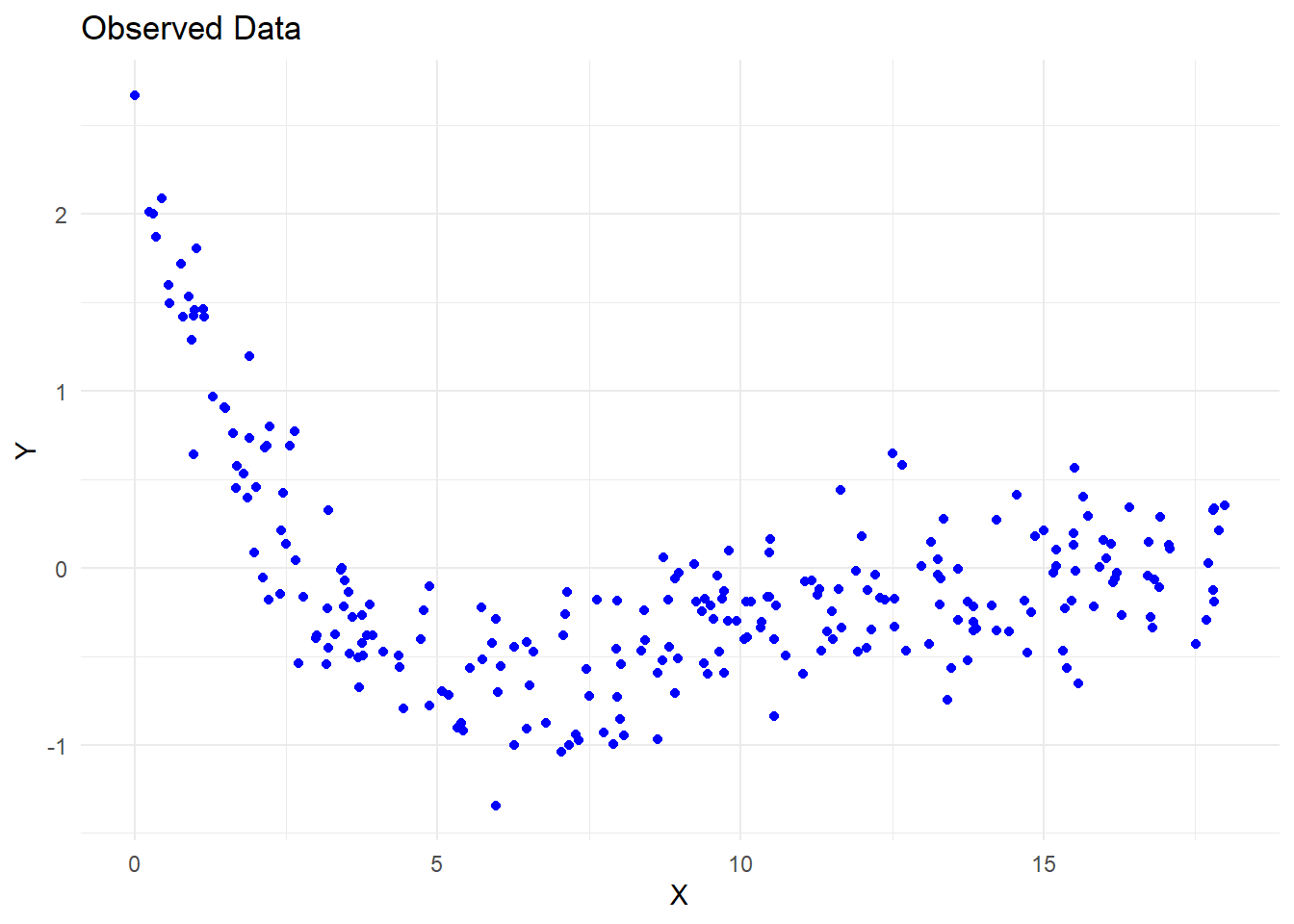

Figure 6.26: Observed Data

2. Deriving Starting Values for Parameters

Since nonlinear optimization is sensitive to starting values, we estimate reasonable initial values based on model interpretation.

Finding the Maximum \(Y\) Value

max(my_data$y)
#> [1] 2.6722
my_data$x[which.max(my_data$y)]
#> [1] 0.0094

• When \(y = 2.6722\), the corresponding \(x = 0.0094\).

• From the model equation: \(\theta_0 + 0.0094 \theta_1 = 2.6722\)

Estimating \(\theta_2\) from the Median \(y\) Value

• The equation simplifies to: \(1 + \theta_2 \exp(0.4 x) = 2\)

# find mean y
mean(my_data$y) 
#> [1] -0.0747864

# find y closest to its mean
my_data$y[which.min(abs(my_data$y - (mean(my_data$y))))] 
#> [1] -0.0773


# find x closest to the mean y
my_data$x[which.min(abs(my_data$y - (mean(my_data$y))))] 
#> [1] 11.0648

• This yields the equation: \(83.58967 \theta_2 = 1\)

Finding the Value of \(\theta_0\) and \(\theta_1\)

# find value of x closet to 1
my_data$x[which.min(abs(my_data$x - 1))] 
#> [1] 0.9895

# find index of x closest to 1
match(my_data$x[which.min(abs(my_data$x - 1))], my_data$x) 
#> [1] 14

# find y value
my_data$y[match(my_data$x[which.min(abs(my_data$x - 1))], my_data$x)]
#> [1] 1.4577

• This provides another equation: \(\theta_0 + \theta_1 \times 0.9895 - 2.164479 \theta_2 = 1.457\)

Solving for \(\theta_0, \theta_1, \theta_2\)

library(matlib)

# Define coefficient matrix
A = matrix(
  c(0, 0.0094, 0, 0, 0, 83.58967, 1, 0.9895, -2.164479),
  nrow = 3,
  ncol = 3,
  byrow = T
)

# Define constant vector
b <- c(2.6722, 1, 1.457)

# Display system of equations
showEqn(A, b)
#> 0*x1 + 0.0094*x2        + 0*x3  =  2.6722 
#> 0*x1      + 0*x2 + 83.58967*x3  =       1 
#> 1*x1 + 0.9895*x2 - 2.164479*x3  =   1.457

# Solve for parameters
theta_start <- Solve(A, b, fractions = FALSE)
#> x1      =  -279.80879739 
#>   x2    =   284.27659574 
#>     x3  =      0.0119632
theta_start
#> [1] "x1      =  -279.80879739" "  x2    =   284.27659574"
#> [3] "    x3  =      0.0119632"

3. Implementing the Gauss-Newton Algorithm

Using these estimates, we manually implement the Gauss-Newton optimization.

Defining the Model and Its Derivatives

# Starting values
theta_0_strt <- as.numeric(gsub(".*=\\s*", "", theta_start[1]))
theta_1_strt <- as.numeric(gsub(".*=\\s*", "", theta_start[2]))
theta_2_strt <- as.numeric(gsub(".*=\\s*", "", theta_start[3]))

# Model function
mod_4 <- function(theta_0, theta_1, theta_2, x) {
  (theta_0 + theta_1 * x) / (1 + theta_2 * exp(0.4 * x))
}

# Define function expression
f_4 = expression((theta_0 + theta_1 * x) / (1 + theta_2 * exp(0.4 * x)))

# First derivatives
df_4.d_theta_0 <- D(f_4, 'theta_0')
df_4.d_theta_1 <- D(f_4, 'theta_1')
df_4.d_theta_2 <- D(f_4, 'theta_2')

Iterative Gauss-Newton Optimization

# Initialize
theta_vec <- matrix(c(theta_0_strt, theta_1_strt, theta_2_strt))
delta <- matrix(NA, nrow = 3, ncol = 1)
i <- 1

# Evaluate function at initial estimates
f_theta <- as.matrix(eval(f_4, list(
  x = my_data$x,
  theta_0 = theta_vec[1, 1],
  theta_1 = theta_vec[2, 1],
  theta_2 = theta_vec[3, 1]
)))

repeat {
  # Compute Jacobian matrix
  F_theta_0 <- as.matrix(cbind(
    eval(df_4.d_theta_0, list(
      x = my_data$x,
      theta_0 = theta_vec[1, i],
      theta_1 = theta_vec[2, i],
      theta_2 = theta_vec[3, i]
    )),
    eval(df_4.d_theta_1, list(
      x = my_data$x,
      theta_0 = theta_vec[1, i],
      theta_1 = theta_vec[2, i],
      theta_2 = theta_vec[3, i]
    )),
    eval(df_4.d_theta_2, list(
      x = my_data$x,
      theta_0 = theta_vec[1, i],
      theta_1 = theta_vec[2, i],
      theta_2 = theta_vec[3, i]
    ))
  ))
  
  # Compute parameter updates
  delta[, i] = (solve(t(F_theta_0)%*%F_theta_0))%*%t(F_theta_0)%*%(my_data$y-f_theta[,i])
    
  
  # Update parameter estimates
  theta_vec <- cbind(theta_vec, theta_vec[, i] + delta[, i])
  theta_vec[, i + 1] = theta_vec[, i] + delta[, i]
  
  # Increment iteration counter
  i <- i + 1
  
  # Compute new function values
  f_theta <- cbind(f_theta, as.matrix(eval(f_4, list(
    x = my_data$x,
    theta_0 = theta_vec[1, i],
    theta_1 = theta_vec[2, i],
    theta_2 = theta_vec[3, i]
  ))))
  
  delta = cbind(delta, matrix(NA, nrow = 3, ncol = 1))
  
  # Convergence criteria based on SSE
  if (abs(sum((my_data$y - f_theta[, i])^2) - sum((my_data$y - f_theta[, i - 1])^2)) / 
      sum((my_data$y - f_theta[, i - 1])^2) < 0.001) {
    break
  }
}

# Final parameter estimates
theta_vec[, ncol(theta_vec)]
#> [1]  3.6335135 -1.3055166  0.5043502

4. Checking Convergence and Variance

# Final objective function value (SSE)
sum((my_data$y - f_theta[, i])^2)
#> [1] 19.80165

sigma2 <- 1 / (nrow(my_data) - 3) * 
  (t(my_data$y - f_theta[, ncol(f_theta)]) %*% 
   (my_data$y - f_theta[, ncol(f_theta)]))  # p = 3

# Asymptotic variance-covariance matrix
as.numeric(sigma2)*as.matrix(solve(crossprod(F_theta_0)))
#>             [,1]        [,2]        [,3]
#> [1,]  0.11552571 -0.04817428  0.02685848
#> [2,] -0.04817428  0.02100861 -0.01158212
#> [3,]  0.02685848 -0.01158212  0.00703916

5. Validating with nls()

nlin_4 <- nls(
  y ~ mod_4(theta_0, theta_1, theta_2, x),
  start = list(
    theta_0 = as.numeric(gsub(".*=\\s*", "", theta_start[1])),
    theta_1 = as.numeric(gsub(".*=\\s*", "", theta_start[2])),
    theta_2 = as.numeric(gsub(".*=\\s*", "", theta_start[3]))
  ),
  data = my_data
)
summary(nlin_4)
#> 
#> Formula: y ~ mod_4(theta_0, theta_1, theta_2, x)
#> 
#> Parameters:
#>         Estimate Std. Error t value Pr(>|t|)    
#> theta_0  3.63591    0.36528   9.954  < 2e-16 ***
#> theta_1 -1.30639    0.15561  -8.395 3.65e-15 ***
#> theta_2  0.50528    0.09215   5.483 1.03e-07 ***
#> ---
#> Signif. codes:  0 '***' 0.001 '**' 0.01 '*' 0.05 '.' 0.1 ' ' 1
#> 
#> Residual standard error: 0.2831 on 247 degrees of freedom
#> 
#> Number of iterations to convergence: 9 
#> Achieved convergence tolerance: 2.307e-07

6.4.2 Logistic Growth Model

A classic logistic growth model follows the equation:

\[ P = \frac{K}{1 + \exp(P_0 + r t)} + \epsilon \]

where:

• \(P\) = population at time \(t\)

• \(K\) = carrying capacity (maximum population)

• \(r\) = population growth rate

• \(P_0\) = initial population log-ratio

However, R’s built-in SSlogis function uses a slightly different parameterization:

\[ P = \frac{asym}{1 + \exp\left(\frac{xmid - t}{scal}\right)} \]

where:

• \(asym\) = carrying capacity (\(K\))

• \(xmid\) = the \(x\)-value at the inflection point of the curve

• \(scal\) = scaling parameter

This gives the parameter relationships:

• \(K = asym\)

• \(r = -1 / scal\)

• \(P_0 = -r \cdot xmid\)

# Simulated time-series data
time <- c(1, 2, 3, 5, 10, 15, 20, 25, 30, 35)
population <- c(2.8, 4.2, 3.5, 6.3, 15.7, 21.3, 23.7, 25.1, 25.8, 25.9)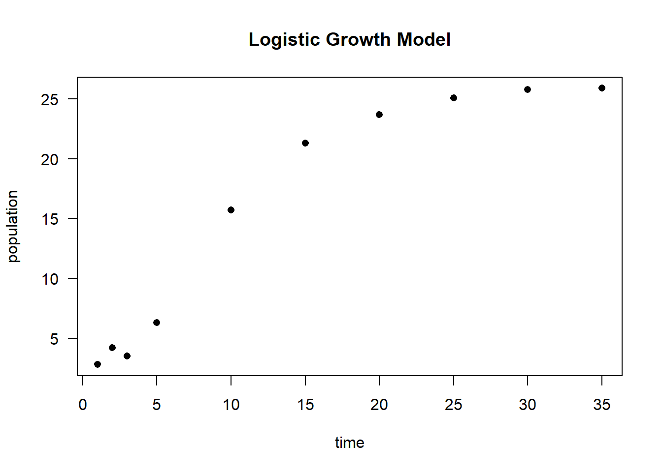

# Plot data points
plot(time,
     population,
     las = 1,
     pch = 16,
     main = "Logistic Growth Model")

Figure 6.27: Logistic Growth Model

# Fit the logistic growth model using programmed starting values
logisticModelSS <- nls(population ~ SSlogis(time, Asym, xmid, scal))

# Model summary
summary(logisticModelSS)
#> 
#> Formula: population ~ SSlogis(time, Asym, xmid, scal)
#> 
#> Parameters:
#>      Estimate Std. Error t value Pr(>|t|)    
#> Asym  25.5029     0.3666   69.56 3.34e-11 ***
#> xmid   8.7347     0.3007   29.05 1.48e-08 ***
#> scal   3.6353     0.2186   16.63 6.96e-07 ***
#> ---
#> Signif. codes:  0 '***' 0.001 '**' 0.01 '*' 0.05 '.' 0.1 ' ' 1
#> 
#> Residual standard error: 0.6528 on 7 degrees of freedom
#> 
#> Number of iterations to convergence: 1 
#> Achieved convergence tolerance: 1.906e-06

# Extract parameter estimates
coef(logisticModelSS)
#>      Asym      xmid      scal 
#> 25.502890  8.734698  3.635333

To fit the model using an alternative parameterization (\(K, r, P_0\)), we convert the estimated coefficients:

# Convert parameter estimates to alternative logistic model parameters
Ks <- as.numeric(coef(logisticModelSS)[1])  # Carrying capacity (K)
rs <- -1 / as.numeric(coef(logisticModelSS)[3])  # Growth rate (r)
Pos <- -rs * as.numeric(coef(logisticModelSS)[2])  # P_0

# Fit the logistic model with the alternative parameterization
logisticModel <- nls(
    population ~ K / (1 + exp(Po + r * time)),
    start = list(Po = Pos, r = rs, K = Ks)
)

# Model summary
summary(logisticModel)
#> 
#> Formula: population ~ K/(1 + exp(Po + r * time))
#> 
#> Parameters:
#>    Estimate Std. Error t value Pr(>|t|)    
#> Po  2.40272    0.12702   18.92 2.87e-07 ***
#> r  -0.27508    0.01654  -16.63 6.96e-07 ***
#> K  25.50289    0.36665   69.56 3.34e-11 ***
#> ---
#> Signif. codes:  0 '***' 0.001 '**' 0.01 '*' 0.05 '.' 0.1 ' ' 1
#> 
#> Residual standard error: 0.6528 on 7 degrees of freedom
#> 
#> Number of iterations to convergence: 0 
#> Achieved convergence tolerance: 1.91e-06

Visualizing the Logistic Model Fit

# Plot original data
plot(time,
     population,
     las = 1,
     pch = 16,
     main = "Logistic Growth Model Fit")

# Overlay the fitted logistic curve
lines(time,
      predict(logisticModel),
      col = "red",
      lwd = 2)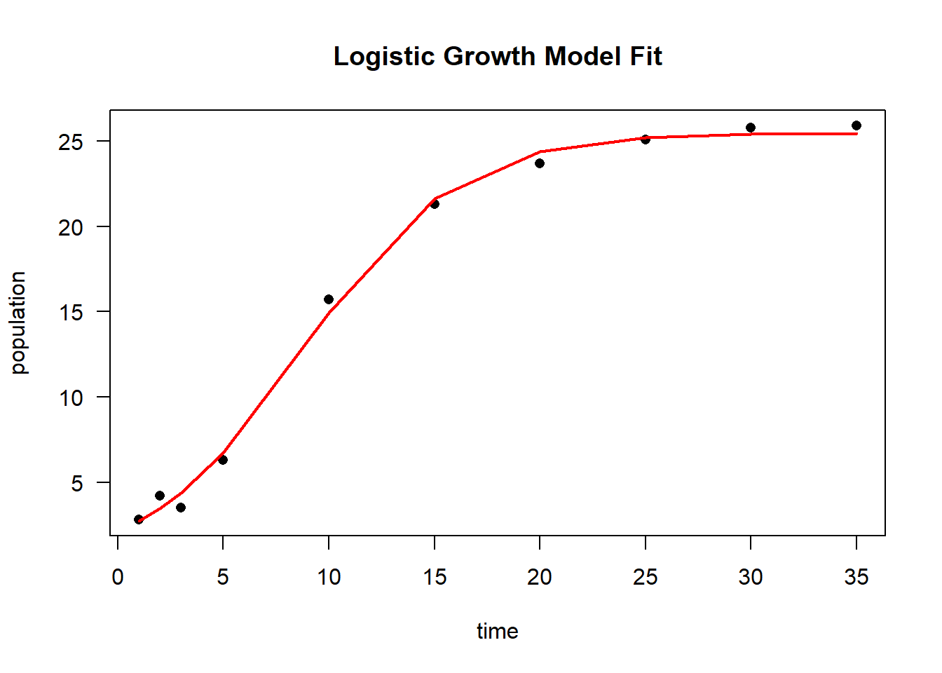

Figure 6.28: Logistic Growth Model Fit

6.4.3 Nonlinear Plateau Model

This example is based on (Schabenberger and Pierce 2001) and demonstrates the use of a plateau model to estimate the relationship between soil nitrate (\(NO_3\)) concentration and relative yield percent (RYP) at two different depths (30 cm and 60 cm).

# Load data
dat <- read.table("images/dat.txt", header = TRUE)

# Plot NO3 concentration vs. relative yield percent, colored by depth
library(ggplot2)
dat.plot <- ggplot(dat) + 
  geom_point(aes(x = no3, y = ryp, color = as.factor(depth))) +
  labs(color = 'Depth (cm)') + 
  xlab('Soil NO3 Concentration') + 
  ylab('Relative Yield Percent') +
  theme_minimal()

# Display plot
dat.plot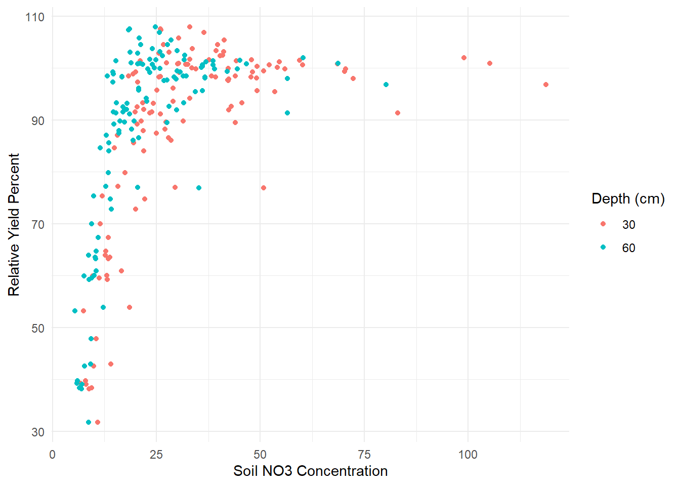

Figure 6.29: Nonlinear Plateau Plot

The suggested nonlinear plateau model is given by:

\[ E(Y_{ij}) = (\beta_{0j} + \beta_{1j}N_{ij})I_{N_{ij}\le \alpha_j} + (\beta_{0j} + \beta_{1j}\alpha_j)I_{N_{ij} > \alpha_j} \]

where:

• \(N_{ij}\) represents the soil nitrate (\(NO_3\)) concentration for observation \(i\) at depth \(j\).

• \(i\) indexes individual observations.

• \(j = 1, 2\) corresponds to depths 30 cm and 60 cm.

This model assumes a linear increase up to a threshold (\(\alpha_j\)), beyond which the response levels off (plateaus).

Defining the Plateau Model as a Function

# Define the nonlinear plateau model function
nonlinModel <- function(predictor, b0, b1, alpha) {
  ifelse(predictor <= alpha, 
         b0 + b1 * predictor,  # Linear growth below threshold
         b0 + b1 * alpha)      # Plateau beyond threshold
}

Creating a Self-Starting Function for nls

Since the model is piecewise linear, we can estimate starting values using:

1. A linear regression on the first half of sorted predictor values to estimate \(b_0\) and \(b_1\).

2. The last predictor value used in the regression as the plateau threshold (\(\alpha\))

# Define initialization function for self-starting plateau model
nonlinModelInit <- function(mCall, LHS, data) {
  # Sort data by increasing predictor value
  xy <- sortedXyData(mCall[['predictor']], LHS, data)
  n <- nrow(xy)
  
  # Fit a simple linear model using the first half of the sorted data
  lmFit <- lm(xy[1:(n / 2), 'y'] ~ xy[1:(n / 2), 'x'])
  
  # Extract initial estimates
  b0 <- coef(lmFit)[1]  # Intercept
  b1 <- coef(lmFit)[2]  # Slope
  alpha <- xy[(n / 2), 'x']  # Last x-value in the fitted linear range
  
  # Return initial parameter estimates
  value <- c(b0, b1, alpha)
  names(value) <- mCall[c('b0', 'b1', 'alpha')]
  value
}

Combining Model and Self-Start Function

# Define a self-starting nonlinear model for nls
SS_nonlinModel <- selfStart(nonlinModel,
                            nonlinModelInit,
                            c('b0', 'b1', 'alpha'))

The nls function is used to estimate parameters separately for each soil depth (30 cm and 60 cm).

# Fit the model for depth = 30 cm
sep30_nls <- nls(ryp ~ SS_nonlinModel(predictor = no3, b0, b1, alpha),
                  data = dat[dat$depth == 30,])

# Fit the model for depth = 60 cm
sep60_nls <- nls(ryp ~ SS_nonlinModel(predictor = no3, b0, b1, alpha),
                  data = dat[dat$depth == 60,])

We generate separate plots for 30 cm and 60 cm depths, showing both confidence and prediction intervals.

# Set plotting layout
par(mfrow = c(1, 2))

# Plot model fit for 30 cm depth
investr::plotFit(
  sep30_nls,
  interval = "both",
  pch = 19,
  shade = TRUE,
  col.conf = "skyblue4",
  col.pred = "lightskyblue2",
  data = dat[dat$depth == 30,],
  main = "Results at 30 cm Depth",
  ylab = "Relative Yield Percent",
  xlab = "Soil NO3 Concentration",
  xlim = c(0, 120)
)

# Plot model fit for 60 cm depth
investr::plotFit(
  sep60_nls,
  interval = "both",
  pch = 19,
  shade = TRUE,
  col.conf = "lightpink4",
  col.pred = "lightpink2",
  data = dat[dat$depth == 60,],
  main = "Results at 60 cm Depth",
  ylab = "Relative Yield Percent",
  xlab = "Soil NO3 Concentration",
  xlim = c(0, 120)
)

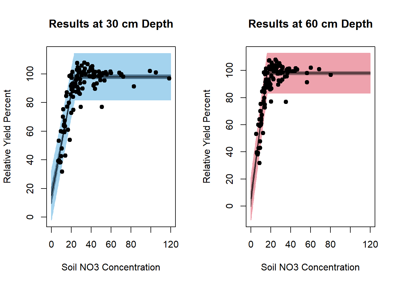
Figure 6.30: Fitted Curves for Relative Yield Response by Soil NO3 Concentration at 30 cm and 60 cm Depths

summary(sep30_nls)
#> 
#> Formula: ryp ~ SS_nonlinModel(predictor = no3, b0, b1, alpha)
#> 
#> Parameters:
#>       Estimate Std. Error t value Pr(>|t|)    
#> b0     15.1943     2.9781   5.102 6.89e-07 ***
#> b1      3.5760     0.1853  19.297  < 2e-16 ***
#> alpha  23.1324     0.5098  45.373  < 2e-16 ***
#> ---
#> Signif. codes:  0 '***' 0.001 '**' 0.01 '*' 0.05 '.' 0.1 ' ' 1
#> 
#> Residual standard error: 8.258 on 237 degrees of freedom
#> 
#> Number of iterations to convergence: 6 
#> Achieved convergence tolerance: 1.166e-08
summary(sep60_nls)
#> 
#> Formula: ryp ~ SS_nonlinModel(predictor = no3, b0, b1, alpha)
#> 
#> Parameters:
#>       Estimate Std. Error t value Pr(>|t|)    
#> b0      5.4519     2.9785    1.83   0.0684 .  
#> b1      5.6820     0.2529   22.46   <2e-16 ***
#> alpha  16.2863     0.2818   57.80   <2e-16 ***
#> ---
#> Signif. codes:  0 '***' 0.001 '**' 0.01 '*' 0.05 '.' 0.1 ' ' 1
#> 
#> Residual standard error: 7.427 on 237 degrees of freedom
#> 
#> Number of iterations to convergence: 5 
#> Achieved convergence tolerance: 2.196e-08

Modeling Soil Depths Together and Comparing Models

Instead of fitting separate models for different soil depths, we first fit a combined model where all observations share a common slope, intercept, and plateau. We then test whether modeling the two depths separately provides a significantly better fit.

1. Fitting a Reduced (Combined) Model

The reduced model assumes that all soil depths follow the same nonlinear relationship.

# Fit the combined model (common parameters across all depths)
red_nls <- nls(
  ryp ~ SS_nonlinModel(predictor = no3, b0, b1, alpha), 
  data = dat
)

# Display model summary
summary(red_nls)
#> 
#> Formula: ryp ~ SS_nonlinModel(predictor = no3, b0, b1, alpha)
#> 
#> Parameters:
#>       Estimate Std. Error t value Pr(>|t|)    
#> b0      8.7901     2.7688   3.175   0.0016 ** 
#> b1      4.8995     0.2207  22.203   <2e-16 ***
#> alpha  18.0333     0.3242  55.630   <2e-16 ***
#> ---
#> Signif. codes:  0 '***' 0.001 '**' 0.01 '*' 0.05 '.' 0.1 ' ' 1
#> 
#> Residual standard error: 9.13 on 477 degrees of freedom
#> 
#> Number of iterations to convergence: 7 
#> Achieved convergence tolerance: 8.568e-09

# Visualizing the combined model fit
par(mfrow = c(1, 1))
plotFit(
  red_nls,
  interval = "both",
  pch = 19,
  shade = TRUE,
  col.conf = "lightblue4",
  col.pred = "lightblue2",
  data = dat,
  main = 'Results for Combined Model',
  ylab = 'Relative Yield Percent',
  xlab = 'Soil NO3 Concentration'
)

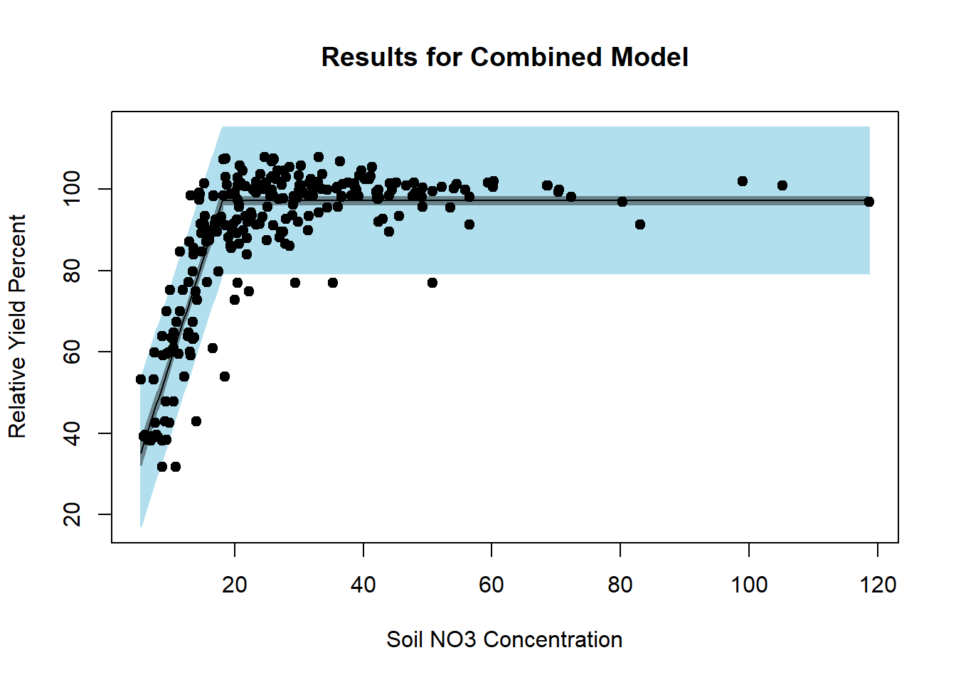
Figure 6.31: Results for Combined Model

2. Examining Residuals for the Combined Model

Checking residuals helps diagnose potential lack of fit.

library(nlstools)

# Residual diagnostics using nlstools
resid <- nlsResiduals(red_nls)

# Plot residuals
plot(resid)

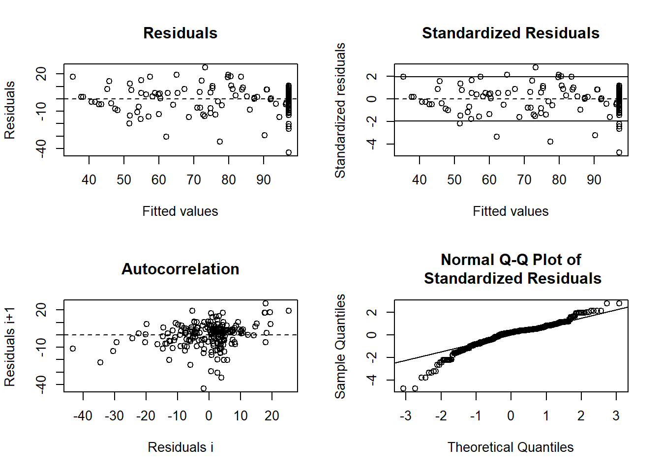
Figure 6.32: Residual Plot Nonlinear Example

If there is a pattern in the residuals (e.g., systematic deviations based on soil depth), this suggests that a separate model for each depth may be necessary.

3. Testing Whether Depths Require Separate Models

To formally test whether soil depth significantly affects the model parameters, we introduce a parameterization where depth-specific parameters are increments from a baseline model (30 cm depth):

\[ \begin{aligned} \beta_{02} &= \beta_{01} + d_0 \\ \beta_{12} &= \beta_{11} + d_1 \\ \alpha_{2} &= \alpha_{1} + d_a \end{aligned} \]

where:

• \(\beta_{01}, \beta_{11}, \alpha_1\) are parameters for 30 cm depth.

• \(d_0, d_1, d_a\) represent depth-specific differences for 60 cm depth.

• If \(d_0, d_1, d_a\) are significantly different from 0, the two depths should be modeled separately.

4. Defining the Full (Depth-Specific) Model

nonlinModelF <- function(predictor, soildep, b01, b11, a1, d0, d1, da) {
  
  # Define parameters for 60 cm depth as increments from 30 cm parameters
  b02 <- b01 + d0
  b12 <- b11 + d1
  a2 <- a1 + da
  
  # Compute model output for 30 cm depth
  y1 <- ifelse(
    predictor <= a1, 
    b01 + b11 * predictor, 
    b01 + b11 * a1
  )
  
  # Compute model output for 60 cm depth
  y2 <- ifelse(
    predictor <= a2, 
    b02 + b12 * predictor, 
    b02 + b12 * a2
  )
  
  # Assign correct model output based on depth
  y <- y1 * (soildep == 30) + y2 * (soildep == 60)
  
  return(y)
}

5. Fitting the Full (Depth-Specific) Model

The starting values are taken from the separately fitted models for each depth.

Soil_full <- nls(
  ryp ~ nonlinModelF(
    predictor = no3,
    soildep = depth,
    b01,
    b11,
    a1,
    d0,
    d1,
    da
  ),
  data = dat,
  start = list(
    b01 = 15.2,   # Intercept for 30 cm depth
    b11 = 3.58,   # Slope for 30 cm depth
    a1 = 23.13,   # Plateau cutoff for 30 cm depth
    d0 = -9.74,   # Intercept difference (60 cm - 30 cm)
    d1 = 2.11,    # Slope difference (60 cm - 30 cm)
    da = -6.85    # Plateau cutoff difference (60 cm - 30 cm)
  )
)

# Display model summary
summary(Soil_full)
#> 
#> Formula: ryp ~ nonlinModelF(predictor = no3, soildep = depth, b01, b11, 
#>     a1, d0, d1, da)
#> 
#> Parameters:
#>     Estimate Std. Error t value Pr(>|t|)    
#> b01  15.1943     2.8322   5.365 1.27e-07 ***
#> b11   3.5760     0.1762  20.291  < 2e-16 ***
#> a1   23.1324     0.4848  47.711  < 2e-16 ***
#> d0   -9.7424     4.2357  -2.300   0.0219 *  
#> d1    2.1060     0.3203   6.575 1.29e-10 ***
#> da   -6.8461     0.5691 -12.030  < 2e-16 ***
#> ---
#> Signif. codes:  0 '***' 0.001 '**' 0.01 '*' 0.05 '.' 0.1 ' ' 1
#> 
#> Residual standard error: 7.854 on 474 degrees of freedom
#> 
#> Number of iterations to convergence: 1 
#> Achieved convergence tolerance: 3.742e-06

6. Model Comparison: Does Depth Matter?

• If \(d_0, d_1, d_a\) are significantly different from 0, the depths should be modeled separately.

• The p-values for these parameters indicate whether depth-specific modeling is necessary.

---

References

Schabenberger, Oliver, and Francis J Pierce. 2001. Contemporary Statistical Models for the Plant and Soil Sciences. CRC press.