5.4 Penalized (Regularized) Estimators
Penalized or regularized estimators are extensions of Ordinary Least Squares designed to address its limitations, particularly in high-dimensional settings. Regularization methods introduce a penalty term to the loss function to prevent overfitting, handle multicollinearity, and improve model interpretability.
There are three popular regularization techniques (but not limited to):
5.4.1 Motivation for Penalized Estimators
OLS minimizes the Residual Sum of Squares (RSS):
\[ RSS = \sum_{i=1}^n \left( y_i - \hat{y}_i \right)^2 = \sum_{i=1}^n \left( y_i - x_i'\beta \right)^2, \]
where:
\(y_i\) is the observed outcome,
\(x_i\) is the vector of predictors for observation \(i\),
\(\beta\) is the vector of coefficients.
While OLS works well under ideal conditions (e.g., low dimensionality, no multicollinearity), it struggles when:
Multicollinearity: Predictors are highly correlated, leading to large variances in \(\beta\) estimates.
High Dimensionality: The number of predictors (\(p\)) exceeds or approaches the sample size (\(n\)), making OLS inapplicable or unstable.
Overfitting: When \(p\) is large, OLS fits noise in the data, reducing generalizability.
To address these issues, penalized regression modifies the OLS loss function by adding a penalty term that shrinks the coefficients toward zero. This discourages overfitting and improves predictive performance.
The general form of the penalized loss function is:
\[ L(\beta) = \sum_{i=1}^n \left( y_i - x_i'\beta \right)^2 + \lambda P(\beta), \]
where:
\(\lambda \geq 0\): Tuning parameter controlling the strength of regularization.
\(P(\beta)\): Penalty term that quantifies model complexity.
Different choices of \(P(\beta)\) lead to ridge regression, lasso regression, or elastic net.
5.4.2 Ridge Regression
Ridge regression, also known as L2 regularization, penalizes the sum of squared coefficients:
\[ P(\beta) = \sum_{j=1}^p \beta_j^2. \]
The ridge objective function becomes:
\[ L_{ridge}(\beta) = \sum_{i=1}^n \left( y_i - x_i'\beta \right)^2 + \lambda \sum_{j=1}^p \beta_j^2, \]
where:
- \(\lambda \geq 0\) controls the degree of shrinkage. Larger \(\lambda\) leads to greater shrinkage.
Ridge regression has a closed-form solution:
\[ \hat{\beta}_{ridge} = \left( X'X + \lambda I \right)^{-1} X'y, \]
where \(I\) is the \(p \times p\) identity matrix.
Key Features
- Shrinks coefficients but does not set them exactly to zero.
- Handles multicollinearity effectively by stabilizing the coefficient estimates (Hoerl and Kennard 1970).
- Works well when all predictors contribute to the response.
Example Use Case
Ridge regression is ideal for applications with many correlated predictors, such as:
- Predicting housing prices based on a large set of features (e.g., size, location, age of the house).
5.4.3 Lasso Regression
Lasso regression, or L1 regularization, penalizes the sum of absolute coefficients:
\[ P(\beta) = \sum_{j=1}^p |\beta_j|. \]
The lasso objective function is:
\[ L_{lasso}(\beta) = \sum_{i=1}^n \left( y_i - x_i'\beta \right)^2 + \lambda \sum_{j=1}^p |\beta_j|. \]
Key Features
- Unlike ridge regression, lasso can set coefficients to exactly zero, performing automatic feature selection.
- Encourages sparse models, making it suitable for high-dimensional data (Tibshirani 1996).
Optimization
Lasso does not have a closed-form solution due to the non-differentiability of \(|\beta_j|\) at \(\beta_j = 0\). It requires iterative algorithms, such as:
Coordinate Descent,
Least Angle Regression (LARS).
Example Use Case
Lasso regression is useful when many predictors are irrelevant, such as:
- Genomics, where only a subset of genes are associated with a disease outcome.
5.4.4 Elastic Net
Elastic Net combines the penalties of ridge and lasso regression:
\[ P(\beta) = \alpha \sum_{j=1}^p |\beta_j| + \frac{1 - \alpha}{2} \sum_{j=1}^p \beta_j^2, \]
where:
\(0 \leq \alpha \leq 1\) determines the balance between lasso (L1) and ridge (L2) penalties.
\(\lambda\) controls the overall strength of regularization.
The elastic net objective function is:
\[ L_{elastic\ net}(\beta) = \sum_{i=1}^n \left( y_i - x_i'\beta \right)^2 + \lambda \left( \alpha \sum_{j=1}^p |\beta_j| + \frac{1 - \alpha}{2} \sum_{j=1}^p \beta_j^2 \right). \]
Key Features
- Combines the strengths of lasso (sparse models) and ridge (stability with correlated predictors) (H. Zou and Hastie 2005).
- Effective when predictors are highly correlated or when \(p > n\).
Example Use Case
Elastic net is ideal for high-dimensional datasets with correlated predictors, such as:
- Predicting customer churn using demographic and behavioral features.
5.4.5 Tuning Parameter Selection
Choosing the regularization parameter \(\lambda\) (and \(\alpha\) for elastic net) is critical for balancing model complexity (fit) and regularization (parsimony). If \(\lambda\) is too large, coefficients are overly shrunk (or even set to zero in the case of L1 penalty), leading to underfitting. If \(\lambda\) is too small, the model might overfit because coefficients are not penalized sufficiently. Hence, a systematic approach is needed to determine the optimal \(\lambda\). For elastic net, we also choose an appropriate \(\alpha\) to balance the L1 and L2 penalties.
5.4.5.1 Cross-Validation
A common approach to selecting \(\lambda\) (and \(\alpha\)) is \(K\)-Fold Cross-Validation:
- Partition the data into \(K\) roughly equal-sized “folds.”
- Train the model on \(K-1\) folds and validate on the remaining fold, computing a validation error.
- Repeat this process for all folds, and compute the average validation error across the \(K\) folds.
- Select the value of \(\lambda\) (and \(\alpha\) if tuning it) that minimizes the cross-validated error.
This method helps us maintain a good bias-variance trade-off because every point is used for both training and validation exactly once.
5.4.5.2 Information Criteria
Alternatively, one can use information criteria—like the Akaike Information Criterion (AIC) or the Bayesian Information Criterion (BIC)—to guide model selection. These criteria reward goodness-of-fit while penalizing model complexity, thereby helping in selecting an appropriately regularized model.
5.4.6 Properties of Penalized Estimators
- Bias-Variance Tradeoff:
- Regularization introduces some bias in exchange for reducing variance, often resulting in better predictive performance on new data.
- Shrinkage:
- Ridge shrinks coefficients toward zero but usually retains all predictors.
- Lasso shrinks some coefficients exactly to zero, performing inherent feature selection.
- Flexibility:
- Elastic net allows for a continuum between ridge and lasso, so it can adapt to different data structures (e.g., many correlated features or very high-dimensional feature spaces).
# Load required libraries
library(glmnet)

# Simulate data
set.seed(123)
n <- 100   # Number of observations
p <- 20    # Number of predictors
X <- matrix(rnorm(n * p), nrow = n, ncol = p)  # Predictor matrix
y <- rnorm(n)                                 # Response vector

# Ridge regression (alpha = 0)
ridge_fit <- glmnet(X, y, alpha = 0)
plot(ridge_fit, xvar = "lambda", label = TRUE)
title("Coefficient Paths for Ridge Regression")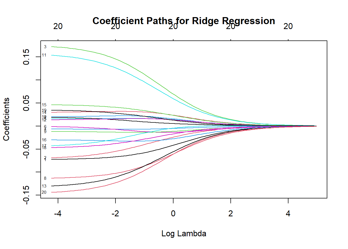
Figure 5.12: Coefficient Paths for Ridge Regression
In this plot, each curve represents a coefficient’s value as a function of \(\lambda\).
As \(\lambda\) increases (moving from left to right on a log-scale by default), coefficients shrink toward zero but typically stay non-zero.
Ridge regression tends to shrink coefficients but does not force them to be exactly zero.
# Lasso regression (alpha = 1)
lasso_fit <- glmnet(X, y, alpha = 1)
plot(lasso_fit, xvar = "lambda", label = TRUE)
title("Coefficient Paths for Lasso Regression")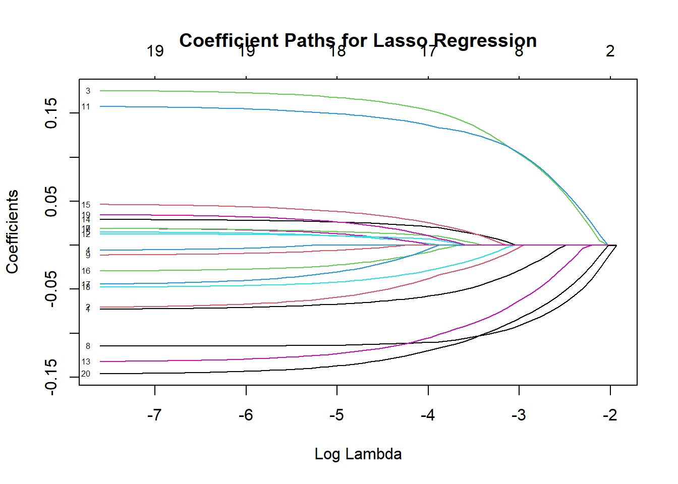
Figure 5.13: Coefficient Paths for Lasso Regression
Here, as \(\lambda\) grows, several coefficient paths hit zero exactly, illustrating the variable selection property of lasso.
# Elastic net (alpha = 0.5)
elastic_net_fit <- glmnet(X, y, alpha = 0.5)
plot(elastic_net_fit, xvar = "lambda", label = TRUE)
title("Coefficient Paths for Elastic Net (alpha = 0.5)")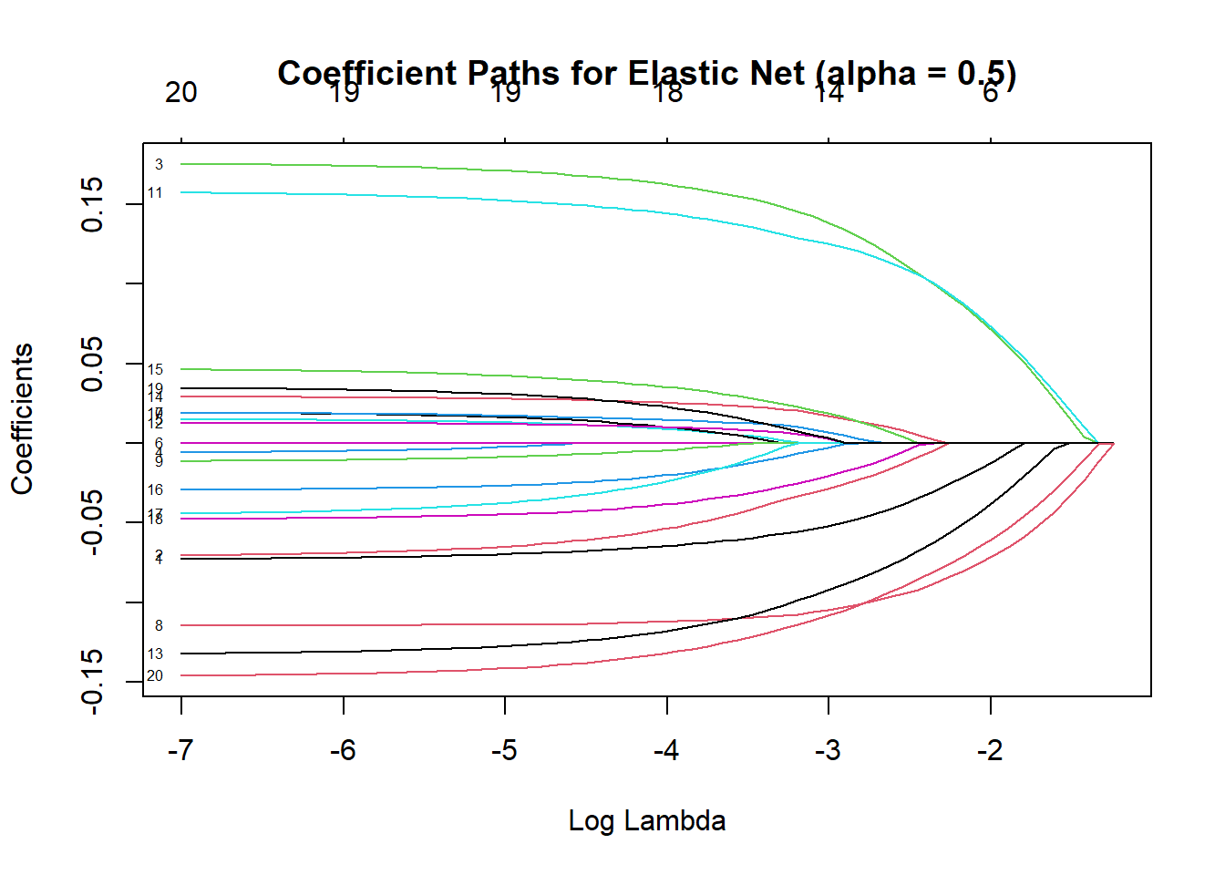
Figure 5.14: Coefficient Paths for Elastic Net
Elastic net combines ridge and lasso penalties. At \(\lambda = 0.5\), we see partial shrinkage and some coefficients going to zero.
This model is often helpful when you suspect both group-wise shrinkage (like ridge) and sparse solutions (like lasso) might be beneficial.
We can further refine our choice of \(\lambda\) by performing cross-validation on the lasso model:
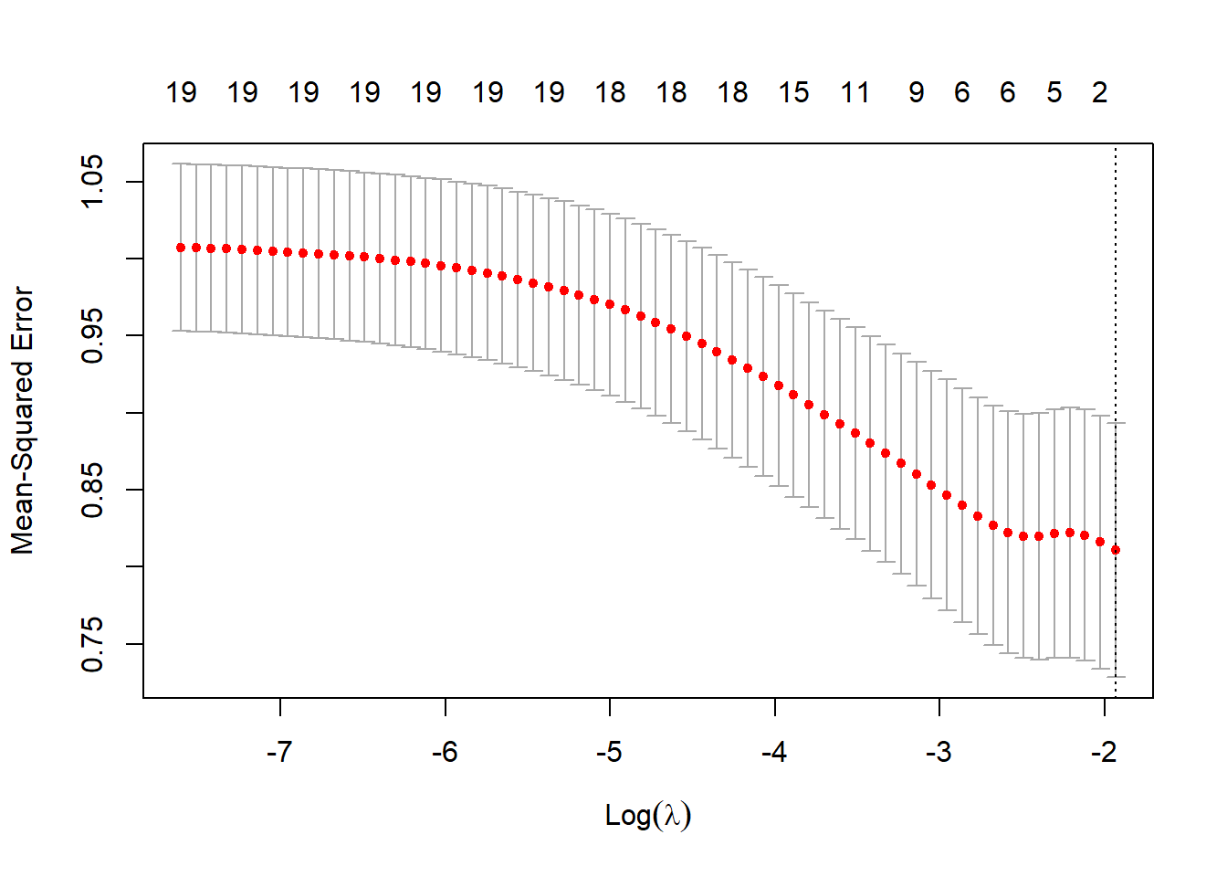
Figure 5.15: Cross-Validation Curve for Lasso Regression: Mean-Squared Error by Log Lambda
The plot displays the cross-validated error (often mean-squared error or deviance) on the y-axis versus \(\log(\lambda)\) on the x-axis.
Two vertical dotted lines typically appear:
\(\lambda.min\): The \(\lambda\) that achieves the minimum cross-validated error.
\(\lambda.1se\): The largest \(\lambda\) such that the cross-validated error is still within one standard error of the minimum. This is a more conservative choice that favors higher regularization (simpler models).
best_lambdaabove prints the numeric value of \(\lambda.min\). This is the \(\lambda\) that gave the lowest cross-validation error for the lasso model.
Interpretation:
By using
cv.glmnet, we systematically compare different values of \(\lambda\) in terms of their predictive performance (cross-validation error).The selected \(\lambda\) typically balances having a smaller model (due to regularization) with retaining sufficient predictive power.
If we used real-world data, we might also look at performance metrics on a hold-out test set to ensure that the chosen \(\lambda\) generalizes well.