27.6 Specification Checks
To validate the credibility of an RD design, researchers perform several specification checks:
- Balance Checks
- Sorting, Bunching, and Manipulation
- Placebo Tests
- Sensitivity to Bandwidth Choice
- Manipulation-Robust Regression Discontinuity Bounds
27.6.1 Balance Checks
Also known as checking for discontinuities in average covariates, this test examines whether covariates that should not be affected by treatment exhibit a discontinuity at the cutoff.
- Null Hypothesis (\(H_0\)): The average effect of covariates on pseudo-outcomes (i.e., those that should not be influenced by treatment) is zero.
- If rejected, this raises serious doubts about the RD design, necessitating a strong justification.
27.6.2 Sorting, Bunching, and Manipulation
This test, also known as checking for discontinuities in the distribution of the forcing variable, detects whether subjects manipulate the running variable to sort into or out of treatment.
If individuals can manipulate the running variable, especially when the cutoff is known in advance, this can lead to bunching behavior (i.e., clustering just above or below the cutoff).
- If treatment is desirable, individuals will try to sort into treatment, leading to a gap just below the cutoff.
- If treatment is undesirable, individuals will try to avoid it, leading to a gap just above the cutoff.
Under RD, we assume that there is no manipulation in the running variable. However, bunching behavior, where firms or individuals strategically manipulate their position, violates this assumption.
To address this issue, the bunching approach estimates the counterfactual distribution, what the density of individuals would have been in the absence of manipulation.
The fraction of individuals who engaged in manipulation is then calculated by comparing the observed distribution to this counterfactual distribution.
In a standard RD framework, this step is unnecessary because it assumes that the observed distribution and the counterfactual (manipulation-free) distribution are the same, implying no manipulation
27.6.2.1 McCrary Sorting Test
A widely used formal test is the McCrary density test (McCrary 2008), later refined by Cattaneo, Idrobo, and Titiunik (2019).
- Null Hypothesis (\(H_0\)): The density of the running variable is continuous at the cutoff.
- Alternative Hypothesis (\(H_a\)): A discontinuity (jump) in the density function at the cutoff, suggesting manipulation.
- Interpretation:
- A significant discontinuity suggests manipulation, violating RD assumptions.
- A failure to reject \(H_0\) does not necessarily confirm validity, as some forms of manipulation may remain undetected.
- If there is two-sided manipulation, this test will fail to detect it.
27.6.2.2 Guidelines for Assessing Manipulation
- J. L. Zhang and Rubin (2003), Lee (2009), and Aronow, Baron, and Pinson (2019) provide criteria for evaluating manipulation risks.
- Knowing your research design inside out is crucial to anticipating possible manipulation attempts.
- Manipulation is often one-sided, meaning subjects shift only in one direction relative to the cutoff. In rare cases, two-sided manipulation may occur but often cancels out.
- We could also observe partial manipulation in reality (e.g., when subjects can only imperfectly manipulate). However, since we typically treat it like a fuzzy RD, we would not encounter identification problems. In contrast, complete manipulation would lead to serious identification issues.
Bunching Methodology
- Bunching occurs when individuals self-select into specific values of the running variable (e.g., policy thresholds). See Kleven (2016) for a review.
- The method helps estimate the counterfactual distribution (what the density would have been without manipulation).
- The fraction of individuals who manipulated can be estimated by comparing observed densities to the counterfactual.
If the running variable and outcome are simultaneously determined, a modified RD estimator can be used for consistent estimation (Bajari et al. 2011):
- One-sided manipulation: Individuals shift only in one direction relative to the cutoff (similar to the monotonicity assumption in instrumental variables).
- Bounded manipulation (regularity assumption): The density of individuals far from the threshold remains unaffected (Blomquist et al. 2021; Bertanha, McCallum, and Seegert 2021).
27.6.2.3 Steps for Bunching Analysis
- Identify the window where bunching occurs (based on Bosch, Dekker, and Strohmaier (2020)). Perform robustness checks by varying the manipulation window.
- Estimate the manipulation-free counterfactual distribution.
- Standard errors for inference can be calculated (following Chetty, Hendren, and Katz (2016)), where bootstrap resampling of residuals is used in estimating the counts of individuals within bins. However, this step may be unnecessary for large datasets.
If the bunching test fails to detect manipulation, we proceed to the Placebo Test.
McCrary Density Test (Discontinuity in Forcing Variable)
Figure 27.1 shows simulated data without discontinuity.
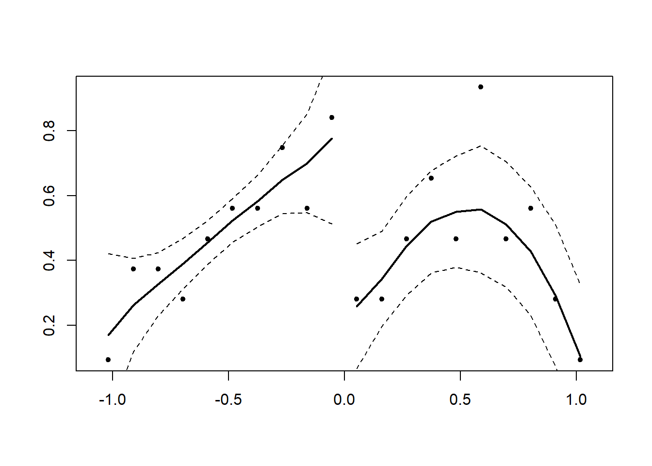
Figure 27.1: Local Polynomial Regression without Discontinuity at Cutoff
#> [1] 0.06355195Figure 27.2 shows simulated data with discontinuity.
# Simulated data with discontinuity
x <- runif(1000, -1, 1)
x <- x + 2 * (runif(1000, -1, 1) > 0 & x < 0)
DCdensity(x, 0)  # Discontinuity detected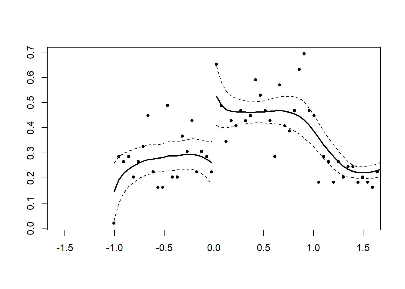
Figure 27.2: Local Polynomial Regression with Discontinuity at Cutoff
#> [1] 0.001936782Cattaneo Density Test (Improved Version)
library(rddensity)

# Simulated continuous density
set.seed(1)
x   <- rnorm(100, mean = -0.5)
rdd <- rddensity(X = x, vce = "jackknife")
summary(rdd)
#>
#> Manipulation testing using local polynomial density estimation.
#>
#> Number of obs =       100
#> Model =               unrestricted
#> Kernel =              triangular
#> BW method =           estimated
#> VCE method =          jackknife
#>
#> c = 0                 Left of c           Right of c
#> Number of obs         66                  34
#> Eff. Number of obs    38                  25
#> Order est. (p)        2                   2
#> Order bias (q)        3                   3
#> BW est. (h)           0.922               0.713
#>
#> Method                T                   P > |T|
#> Robust                0.6715              0.5019
#>
#>
#> P-values of binomial tests (H0: p=0.5).
#>
#> Window Length              <c     >=c    P>|T|
#> 0.563     + 0.563          26      20    0.4614
#> 0.603     + 0.580          27      20    0.3817
#> 0.643     + 0.596          30      20    0.2026
#> 0.683     + 0.613          32      21    0.1690
#> 0.722     + 0.630          32      22    0.2203
#> 0.762     + 0.646          33      22    0.1770
#> 0.802     + 0.663          33      23    0.2288
#> 0.842     + 0.680          35      24    0.1925
#> 0.882     + 0.696          36      24    0.1550
#> 0.922     + 0.713          38      25    0.1299

# Plot requires customization (refer to package documentation)
# rdplotdensity(rdd, x,
#               xlabel = "Running Variable",
#               ylabel = "Density")
27.6.3 Placebo Tests
Placebo tests, also known as falsification checks, assess whether discontinuities appear at points other than the treatment cutoff. This helps verify that observed effects are causal rather than artifacts of the method or data.
- There should be no jumps in the outcome at values other than the cutoff (\(X_i < c\) or \(X_i \geq c\)).
- The test involves shifting the cutoff along the running variable while using the same bandwidth to check for discontinuities in the conditional mean of the outcome.
- This approach is similar to balance checks in experimental design, ensuring no pre-existing differences. Remember, we can only test on observables, not unobservables.
Under a valid RD design, matching methods are unnecessary. Just as with randomized experiments, balance should naturally occur across the threshold. If adjustments are required, it suggests the RD assumptions may be invalid.
27.6.3.1 Applications of Placebo Tests
- Testing No Discontinuity in Predetermined Covariates: Covariates that should not be affected by treatment should not exhibit a jump at the cutoff.
- Testing Other Discontinuities: Checking for discontinuities at other arbitrary points along the running variable.
- Using Placebo Outcomes: If an outcome variable that should not be affected by treatment shows a significant discontinuity, this raises concerns about RD validity.
- Assessing Sensitivity to Covariates: RD estimates should not be highly sensitive to the inclusion or exclusion of covariates.
27.6.3.2 Mathematical Specification
The balance of observable characteristics on both sides of the threshold can be tested using:
\[ Z_i = \alpha_0 + \alpha_1 f(X_i) + I(X_i \geq c) \alpha_2 + [f(X_i) \times I(X_i \geq c)]\alpha_3 + u_i \]
where:
\(X_i\) = running variable
\(Z_i\) = predetermined characteristics (e.g., age, education, etc.)
\(\alpha_2\) should be zero if \(Z_i\) is unaffected by treatment.
If multiple covariates \(Z_i\) are tested simultaneously, simulating their joint distribution avoids false positives due to multiple comparisons. This step is unnecessary if covariates are independent, but such independence is unlikely in practice.
27.6.4 Sensitivity to Bandwidth Choice
The choice of bandwidth is crucial in RD estimation. Different bandwidth selection methods exist:
- Ad-hoc or Substantively Driven: Based on theoretical or empirical reasoning.
- Data-Driven Selection (Cross-Validation): Optimizes bandwidth to minimize prediction error.
- Conservative Approach: Uses robust optimal bandwidth selection methods (e.g., (Calonico, Cattaneo, and Farrell 2020)).
The objective is to minimize mean squared error (MSE) between estimated and actual treatment effects.
27.6.5 Assessing Sensitivity
- Results should be consistent across reasonable bandwidth choices.
- The optimal bandwidth for estimating treatment effects may differ from the optimal bandwidth for testing covariates but should be fairly close.
# Load required package
library(rdd)

# Simulate some data
set.seed(123)
n <- 100  # Sample size

# Running variable centered around 0
running_var <- runif(n, -1, 1)

# Treatment assigned at cutpoint 0
treatment   <- ifelse(running_var >= 0, 1, 0)

# Outcome variable
outcome_var <- 2 * running_var + treatment * 1.5 + rnorm(n)

# Compute the optimal Imbens-Kalyanaraman bandwidth
bandwidth <-
    IKbandwidth(running_var,
                outcome_var,
                cutpoint = 0,
                kernel = "triangular")

# Print the bandwidth
print(bandwidth)
#> [1] 0.4374142
27.6.6 Manipulation-Robust Regression Discontinuity Bounds
Regression Discontinuity designs rely on the assumption that the running variable \(X_i\) is not manipulable by agents in the study. However, McCrary (2008) showed that a discontinuity in the density of \(X_i\) at the cutoff may indicate manipulation, potentially invalidating RD estimates. The common approach to handling detected manipulation is:
- If no manipulation is detected, proceed with RD analysis.
- If manipulation is detected, use the “doughnut-hole” method (i.e., excluding near-cutoff observations), but this contradicts the RD principles (Table 27.2).
However, strict adherence to this rule can lead to two problems:
- False Negatives: A small sample size might fail to detect manipulation, leading to biased estimates if manipulation still affects the running variable.
- Loss of Informative Data: Even when manipulation is detected, the data may still contain valuable information for causal inference.
To address these challenges, Gerard, Rokkanen, and Rothe (2020) introduce a framework that accounts for manipulated observations rather than discarding them. This approach:
- Identifies the extent of manipulation.
- Computes worst-case bounds on treatment effects.
- Provides a systematic way to incorporate manipulated observations while maintaining the credibility of RD analysis.
If manipulation is believed to be unlikely, an alternative approach is to conduct sensitivity analysis by:
Testing how different hypothetical values of \(\tau\) affect the bounds.
Comparing results across various \(\tau\) assumptions to assess robustness.
Consider independent observations \((X_i, Y_i, D_i)\):
- \(X_i\): Running variable.
- \(Y_i\): Outcome variable.
- \(D_i\): Treatment indicator (\(D_i = 1\) if \(X_i \geq c\), and \(D_i = 0\) otherwise).
A sharp RD design satisfies \(D_i = I(X_i \geq c)\), while a fuzzy RD design allows probabilistic treatment assignment.
The population consists of two types of units:
- Potentially-Assigned Units (\(M_i = 0\)): These units follow the standard RD framework. They have potential outcomes \(Y_i(d)\) and potential treatment states \(D_i(x)\).
- Always-Assigned Units (\(M_i = 1\)): These units always appear on one side of the cutoff and do not require potential outcomes.
If no always-assigned units exist (\(M_i = 1\) for no units), the standard RD model holds.
27.6.6.1 Key Assumptions
- Local Independence and Continuity:
- Treatment probability jumps at \(c\) among potentially-assigned units: \[ P(D = 1|X = c^+, M = 0) > P(D = 1|X = c^-, M = 0). \]
- No defiers: \(P(D^+ \geq D^- | X = c, M = 0) = 1\).
- Potential outcomes and treatment states are continuous at \(c\).
- The density of the running variable among potentially-assigned units, \(F_{X|M=0}(x)\), is differentiable at \(c\).
- Smoothness of the Running Variable among Potentially-Assigned Units:
- The derivative of \(F_{X|M=0}(x)\) is continuous at \(c\).
- Restrictions on Always-Assigned Units:
- Always-assigned units satisfy \(P(X \geq c|M = 1) = 1\).
- The density of the running variable among always-assigned units, \(F_{X|M=1}(x)\), is right-differentiable at \(c\).
- This one-sided manipulation assumption allows identification of the proportion of always-assigned units.
When always-assigned units exist, the RD design effectively becomes fuzzy, since: 1. Some potentially-assigned units receive treatment while others do not. 2. Always-assigned units are always treated (or always untreated).
27.6.6.2 Estimating Treatment Effects
For potentially-assigned units, the causal effect of interest is:
\[ \Gamma = E[Y(1) - Y(0) | X = c, D^+ > D^-, M = 0]. \]
This parameter represents the local average treatment effect for potentially-assigned compliers, i.e., those whose treatment status is affected by their running variable crossing the cutoff.
27.6.6.3 Bounding Treatment Effects
The approach to bounding treatment effects consists of two key steps:
- Estimating the Proportion of Always-Assigned Units:
- This is done by measuring the discontinuity in the density of \(X\) at \(c\).
- The larger the discontinuity, the greater the fraction of always-assigned units.
- Computing Worst-Case Bounds on Treatment Effects:
- If manipulation exists, treatment effects must be inferred using extreme-case scenarios.
- For sharp RD designs, bounds are estimated by trimming extreme outcomes near the cutoff.
- For fuzzy RD designs, additional adjustments are required to account for the presence of always-assigned units.
Extensions of this approach use covariates and economic behavior assumptions to refine bounds further.
| Manipulation-Robust RD | Doughnut-Hole RD |
|---|---|
| Uses actual observed data at the cutoff. | Excludes observations near the cutoff. |
| Provides a direct estimate of causal effects. | Relies on extrapolation from other regions. |
| Accounts for manipulation explicitly. | Assumes a hypothetical counterfactual world. |
| Less sensitive to assumptions about manipulation. | Requires strong assumptions about bias. |
27.6.6.4 Identification Challenges
A central challenge in manipulation-robust RD designs is the inability to directly distinguish always-assigned from potentially-assigned units. As a result, the LATE \(\Gamma\) is not point identified. Instead, we establish sharp bounds on \(\Gamma\).
These bounds leverage the stochastic dominance of potential outcome cumulative distribution functions over observed distributions. This allows us to infer treatment effects without making strong parametric assumptions.
To formalize the population structure, we define five types of units:
- Potentially-Assigned Units:
- \(C_0\) (Compliers): Receive treatment if and only if \(X \geq c\).
- \(A_0\) (Always-Takers): Always receive treatment, regardless of \(X\).
- \(N_0\) (Never-Takers): Never receive treatment, regardless of \(X\).
- Always-Assigned Units:
- \(T_1\) (Treated Always-Assigned Units): Always appear above the cutoff and receive treatment.
- \(U_1\) (Untreated Always-Assigned Units): Always appear below the cutoff and do not receive treatment.
The measure \(\tau\), representing the proportion of always-assigned units near the cutoff, is point-identified using the discontinuity in the density of the running variable \(f_X\) at \(c\).
27.6.6.4.1 Identification in Sharp RD
In a sharp RD design:
- Units to the left of the cutoff are potentially-assigned units.
- The observed distribution of untreated outcomes, \(Y(0)\), among these units corresponds to the outcomes of potentially-assigned compliers (\(C_0\)) at the cutoff.
- To estimate sharp bounds on \(\Gamma\), we need to assess the distribution of treated outcomes (\(Y(1)\)) for compliers.
However, information on treated outcomes (\(Y(1)\)) at the cutoff is only available from the treated subpopulation, which includes:
Potentially-assigned compliers (\(C_0\))
Always-assigned treated units (\(T_1\))
Since \(\tau\) is point-identified, we can construct sharp bounds on \(\Gamma\) by adjusting for the presence of \(T_1\).
27.6.6.4.2 Identification in Fuzzy RD
In fuzzy RD, treatment assignment is not deterministic.
- Unit Types and Combinations: There are five distinct unit types and four combinations of treatment assignments and decisions relevant to the analysis. These distinctions are important because they affect how potential outcomes are analyzed and bounded.
- Outcome Distributions: The analysis involves estimating the distribution of potential outcomes (both treated and untreated) among potentially-assigned compliers at the cutoff.
- The goal is to estimate the distribution of potential outcomes (both treated and untreated) for potentially-assigned compliers at the cutoff.
27.6.6.5 Three-Step Process for Bounding Treatment Effects
The method to obtain sharp bounds on \(\Gamma\) follows three steps:
- Bounding Potential Outcomes Under Treatment:
- Use observed treated outcomes to estimate the upper and lower bounds on \(F_{Y(1)}(y | X = c, M = 0)\).
- Bounding Potential Outcomes Under Non-Treatment:
- Use observed untreated outcomes to estimate the upper and lower bounds on \(F_{Y(0)}(y | X = c, M = 0)\).
- Deriving Bounds on \(\Gamma\):
- Using the bounds from Steps 1 and 2, compute sharp upper and lower bounds on the local average treatment effect.
Extreme Value Consideration:
- The bounds account for worst-case scenarios by considering extreme assumptions about the distribution of potential outcomes.
- These bounds are sharp (i.e., they cannot be tightened further without additional assumptions) but remain empirically relevant.
27.6.6.6 Extensions
- Quantile Treatment Effects (QTEs)
An alternative to average treatment effects is the quantile treatment effect (QTE), which focuses on different percentiles of the outcome distribution. Advantages of QTE bounds include:
- Less Sensitivity to Extreme Values: Unlike ATE bounds, QTE bounds are less affected by outliers in the outcome distribution.
- More Informative for Policy Analysis: Helps determine whether effects are concentrated in certain segments of the population.
QTE vs. ATE Under Manipulation:
- ATE inference is highly sensitive to manipulation, with confidence intervals widening significantly as assumed manipulation increases.
- QTE inference remains meaningful even under substantial manipulation.
- Discrete Outcome Extensions: The framework applies not only to continuous outcomes but also to discrete outcome variables.
- Role of Behavioral Assumptions
- Making behavioral assumptions about high treatment likelihood among always-assigned units can refine the bounds.
- For example, assuming that most always-assigned units are treated allows for narrower bounds on treatment effects.
- Incorporation of Covariates
- Including pre-treatment covariates can refine treatment effect bounds.
- Covariates help:
- Distinguish between potentially-assigned and always-assigned units.
- Improve inference on treatment effect heterogeneity.
- Guide policy targeting by identifying unit types based on observed characteristics.
library(formattable)
library(data.table)
library(rdbounds)
set.seed(123)
df <- rdbounds_sampledata(1000, covs = FALSE)
#> [1] "True tau: 0.117999815082062"
#> [1] "True treatment effect on potentially-assigned: 2"
#> [1] "True treatment effect on right side of cutoff: 2.35399944524618"
head(df)
#>            x         y treatment
#> 1 -1.2532616  2.684827         0
#> 2 -0.5146925  5.845219         0
#> 3  3.4853777  6.166070         0
#> 4  0.1576616  3.227139         0
#> 5  0.2890962  7.031685         1
#> 6  3.8350019 10.238570         1

rdbounds_est <-
    rdbounds(
        y = df$y,
        x = df$x,
        # covs = as.factor(df$cov),
        treatment = df$treatment,
        c = 0,
        discrete_x = FALSE,
        discrete_y = FALSE,
        bwsx = c(.2, .5),
        bwy = 1,

        # for median effect use
        # type = "qte",
        # percentiles = .5,

        kernel = "epanechnikov",
        orders = 1,
        evaluation_ys = seq(from = 0, to = 15, by = 1),
        refinement_A = TRUE,
        refinement_B = TRUE,
        right_effects = TRUE,
        yextremes = c(0, 15),
        num_bootstraps = 5
    )
#> [1] "The proportion of always-assigned units just to the right of the cutoff is estimated to be 0.38047"
#> [1] "2025-11-04 09:27:50.247255 Estimating CDFs for point estimates"
#> [1] "2025-11-04 09:27:50.444951 .....Estimating CDFs for units just to the right of the cutoff"
#> [1] "2025-11-04 09:27:52.273855 Estimating CDFs with nudged tau (tau_star)"
#> [1] "2025-11-04 09:27:52.314649 .....Estimating CDFs for units just to the right of the cutoff"
#> [1] "2025-11-04 09:27:55.210347 Beginning parallelized output by bootstrap.."
#> [1] "2025-11-04 09:27:59.760454 Computing Confidence Intervals"
#> [1] "2025-11-04 09:28:11.395259 Time taken:0.35 minutes"rdbounds_summary(rdbounds_est, title_prefix = "Sample Data Results")
#> [1] "Time taken: 0.35 minutes"
#> [1] "Sample size: 1000"
#> [1] "Local Average Treatment Effect:"
#> $tau_hat
#> [1] 0.3804665
#>
#> $tau_hat_CI
#> [1] 0.4180576 1.4333618
#>
#> $takeup_increase
#> [1] 0.6106973
#>
#> $takeup_increase_CI
#> [1] 0.4332132 0.7881814
#>
#> $TE_SRD_naive
#> [1] 1.589962
#>
#> $TE_SRD_naive_CI
#> [1] 1.083977 2.095948
#>
#> $TE_SRD_bounds
#> [1] 0.7165801 2.3454868
#>
#> $TE_SRD_CI
#> [1] -1.200992 7.733214
#>
#> $TE_SRD_covs_bounds
#> [1] NA NA
#>
#> $TE_SRD_covs_CI
#> [1] NA NA
#>
#> $TE_FRD_naive
#> [1] 2.583271
#>
#> $TE_FRD_naive_CI
#> [1] 1.506573 3.659969
#>
#> $TE_FRD_bounds
#> [1] 1.273896 3.684860
#>
#> $TE_FRD_CI
#> [1] -1.266341 10.306116
#>
#> $TE_FRD_bounds_refinementA
#> [1] 1.273896 3.684860
#>
#> $TE_FRD_refinementA_CI
#> [1] -1.266341 10.306116
#>
#> $TE_FRD_bounds_refinementB
#> [1] 1.420594 3.677963
#>
#> $TE_FRD_refinementB_CI
#> [1] NA NA
#>
#> $TE_FRD_covs_bounds
#> [1] NA NA
#>
#> $TE_FRD_covs_CI
#> [1] NA NA
#>
#> $TE_SRD_CIs_manipulation
#> [1] NA NA
#>
#> $TE_FRD_CIs_manipulation
#> [1] NA NA
#>
#> $TE_SRD_right_bounds
#> [1] -2.056178 3.650820
#>
#> $TE_SRD_right_CI
#> [1] -11.044937 9.282217
#>
#> $TE_FRD_right_bounds
#> [1] -2.900703 5.272370
#>
#> $TE_FRD_right_CI
#> [1] -14.75421 15.58640rdbounds_est_tau <-
rdbounds(
y = df$y,
x = df$x,
# covs = as.factor(df$cov),
treatment = df$treatment,
c = 0,
discrete_x = FALSE,
discrete_y = FALSE,
bwsx = c(.2, .5),
bwy = 1,
kernel = "epanechnikov",
orders = 1,
evaluation_ys = seq(from = 0, to = 15, by = 1),
refinement_A = TRUE,
refinement_B = TRUE,
right_effects = TRUE,
potential_taus = c(.025, .05, .1, .2),
yextremes = c(0, 15),
num_bootstraps = 5
)
#> [1] "The proportion of always-assigned units just to the right of the cutoff is estimated to be 0.38047"
#> [1] "2025-11-04 09:28:12.885175 Estimating CDFs for point estimates"
#> [1] "2025-11-04 09:28:13.09748 .....Estimating CDFs for units just to the right of the cutoff"
#> [1] "2025-11-04 09:28:14.953451 Estimating CDFs with nudged tau (tau_star)"
#> [1] "2025-11-04 09:28:14.993297 .....Estimating CDFs for units just to the right of the cutoff"
#> [1] "2025-11-04 09:28:17.846789 Beginning parallelized output by bootstrap.."
#> [1] "2025-11-04 09:28:22.689488 Estimating CDFs with fixed tau value of: 0.025"
#> [1] "2025-11-04 09:28:22.761353 Estimating CDFs with fixed tau value of: 0.05"
#> [1] "2025-11-04 09:28:22.801681 Estimating CDFs with fixed tau value of: 0.1"
#> [1] "2025-11-04 09:28:22.842152 Estimating CDFs with fixed tau value of: 0.2"
#> [1] "2025-11-04 09:28:23.877805 Beginning parallelized output by bootstrap x fixed tau.."
#> [1] "2025-11-04 09:28:26.637232 Computing Confidence Intervals"
#> [1] "2025-11-04 09:28:37.92136 Time taken:0.42 minutes"Figure 27.3 shows the average treatment effect across different shares of always-assigned units.
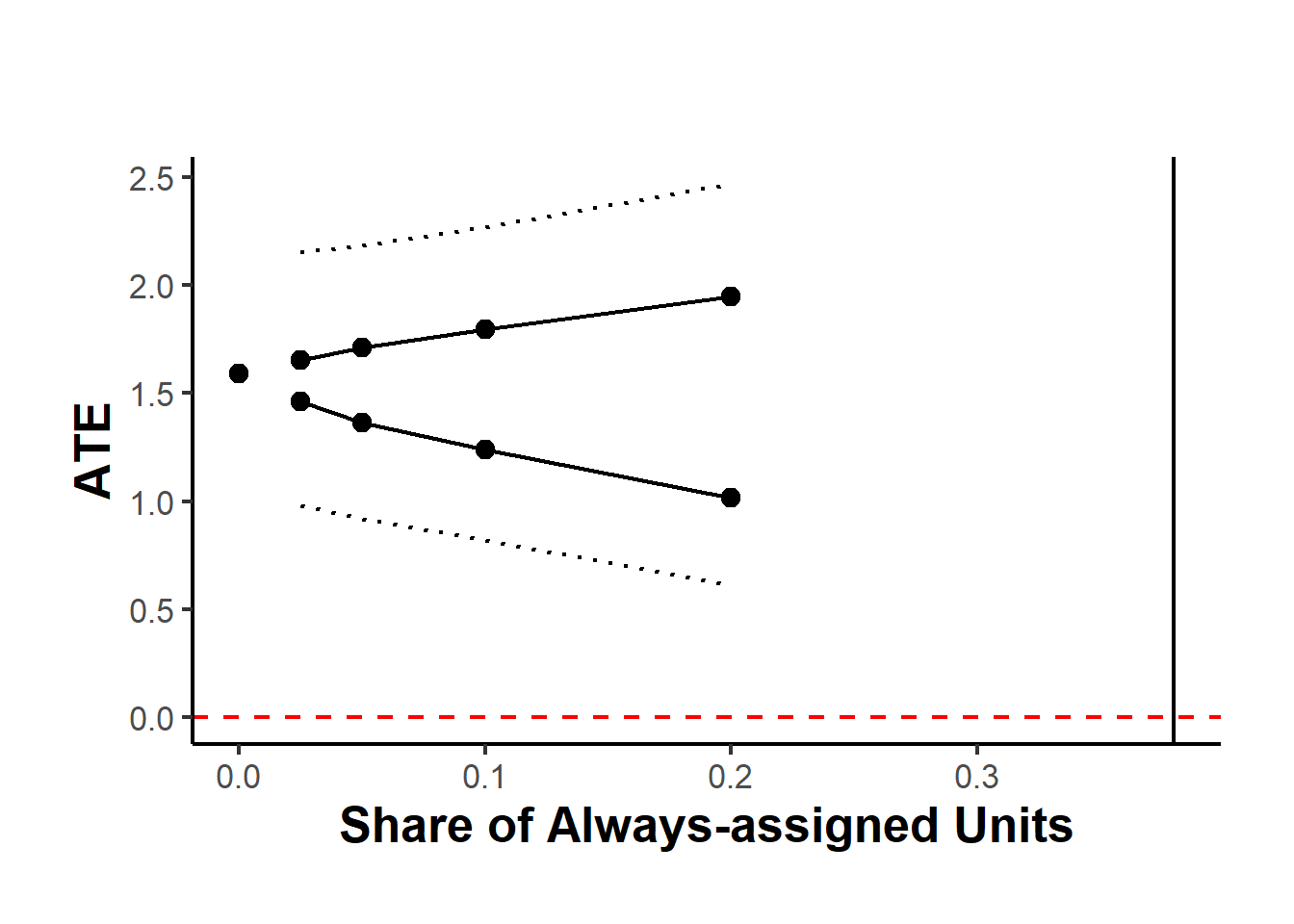
Figure 27.3: Robustness of Average Treatment Effect to Share of Always-assigned Units