7.1 Logistic Regression
Logistic regression is a widely used Generalized Linear Model designed for modeling binary response variables. It is particularly useful in applications such as credit scoring, medical diagnosis, and customer churn prediction.
7.1.1 Logistic Model
Given a set of predictor variables \(\mathbf{x}_i\), the probability of a positive outcome (e.g., success, event occurring) is modeled as:
\[ p_i = f(\mathbf{x}_i ; \beta) = \frac{\exp(\mathbf{x_i'\beta})}{1 + \exp(\mathbf{x_i'\beta})} \]
where:
- \(p_i = \mathbb{E}[Y_i]\) is the probability of success for observation \(i\).
- \(\mathbf{x_i}\) is the vector of predictor variables.
- \(\beta\) is the vector of model coefficients.
7.1.1.1 Logit Transformation
The logistic function can be rewritten in terms of the log-odds, also known as the logit function:
\[ \text{logit}(p_i) = \log \left(\frac{p_i}{1 - p_i} \right) = \mathbf{x_i'\beta} \]
where:
- \(\frac{p_i}{1 - p_i}\) represents the odds of success (the ratio of the probability of success to the probability of failure).
- The logit function ensures linearity in the parameters, which aligns with the GLM framework.
Thus, logistic regression belongs to the family of Generalized Linear Models because a function of the mean response (logit) is linear in the predictors.
7.1.2 Likelihood Function
Since \(Y_i\) follows a Bernoulli distribution with probability \(p_i\), the likelihood function for \(n\) independent observations is:
\[ L(p_i) = \prod_{i=1}^{n} p_i^{Y_i} (1 - p_i)^{1 - Y_i} \]
By substituting the logistic function for \(p_i\):
\[ p_i = \frac{\exp(\mathbf{x'_i \beta})}{1+\exp(\mathbf{x'_i \beta})}, \quad 1 - p_i = \frac{1}{1+\exp(\mathbf{x'_i \beta})} \]
we obtain:
\[ L(\beta) = \prod_{i=1}^{n} \left( \frac{\exp(\mathbf{x'_i \beta})}{1+\exp(\mathbf{x'_i \beta})} \right)^{Y_i} \left( \frac{1}{1+\exp(\mathbf{x'_i \beta})} \right)^{1 - Y_i} \]
Taking the natural logarithm of the likelihood function gives the log-likelihood function:
\[ Q(\beta) = \log L(\beta) = \sum_{i=1}^n Y_i \mathbf{x'_i \beta} - \sum_{i=1}^n \log(1 + \exp(\mathbf{x'_i \beta})) \]
Since this function is concave, we can maximize it numerically using iterative optimization techniques, such as:
- Newton-Raphson Algorithm
- Fisher Scoring Algorithm
These methods allow us to obtain the Maximum Likelihood Estimates of the parameters, \(\hat{\beta}\).
Under standard regularity conditions, the MLEs of logistic regression parameters are asymptotically normal:
\[ \hat{\beta} \dot{\sim} AN(\beta, [\mathbf{I}(\beta)]^{-1}) \]
where:
- \(\mathbf{I}(\beta)\) is the Fisher Information Matrix, which determines the variance-covariance structure of \(\hat{\beta}\).
7.1.3 Fisher Information Matrix
The Fisher Information Matrix quantifies the amount of information that an observable random variable carries about the unknown parameter \(\beta\). It is crucial in estimating the variance-covariance matrix of the estimated coefficients in logistic regression.
Mathematically, the Fisher Information Matrix is defined as:
\[ \mathbf{I}(\beta) = E\left[ \frac{\partial \log L(\beta)}{\partial \beta} \frac{\partial \log L(\beta)}{\partial \beta'} \right] \]
which expands to:
\[ \mathbf{I}(\beta) = E\left[ \left(\frac{\partial \log L(\beta)}{\partial \beta_i} \frac{\partial \log L(\beta)}{\partial \beta_j} \right)_{ij} \right] \]
Under regularity conditions, the Fisher Information Matrix is equivalent to the negative expected Hessian matrix:
\[ \mathbf{I}(\beta) = -E\left[ \frac{\partial^2 \log L(\beta)}{\partial \beta \partial \beta'} \right] \]
which further expands to:
\[ \mathbf{I}(\beta) = -E \left[ \left( \frac{\partial^2 \log L(\beta)}{\partial \beta_i \partial \beta_j} \right)_{ij} \right] \]
This representation is particularly useful because it allows us to compute the Fisher Information Matrix directly from the Hessian of the log-likelihood function.
Example: Fisher Information Matrix in Logistic Regression
Consider a simple logistic regression model with one predictor:
\[ x_i' \beta = \beta_0 + \beta_1 x_i \]
From the log-likelihood function, the second-order partial derivatives are:
\[ \begin{aligned} - \frac{\partial^2 \ln(L(\beta))}{\partial \beta^2_0} &= \sum_{i=1}^n \frac{\exp(x'_i \beta)}{1 + \exp(x'_i \beta)} - \left[\frac{\exp(x_i' \beta)}{1+ \exp(x'_i \beta)}\right]^2 & \text{Intercept} \\ &= \sum_{i=1}^n p_i (1-p_i) \\ - \frac{\partial^2 \ln(L(\beta))}{\partial \beta^2_1} &= \sum_{i=1}^n \frac{x_i^2\exp(x'_i \beta)}{1 + \exp(x'_i \beta)} - \left[\frac{x_i\exp(x_i' \beta)}{1+ \exp(x'_i \beta)}\right]^2 & \text{Slope}\\ &= \sum_{i=1}^n x_i^2p_i (1-p_i) \\ - \frac{\partial^2 \ln(L(\beta))}{\partial \beta_0 \partial \beta_1} &= \sum_{i=1}^n \frac{x_i\exp(x'_i \beta)}{1 + \exp(x'_i \beta)} - x_i\left[\frac{\exp(x_i' \beta)}{1+ \exp(x'_i \beta)}\right]^2 & \text{Cross-derivative}\\ &= \sum_{i=1}^n x_ip_i (1-p_i) \end{aligned} \]
Combining these elements, the Fisher Information Matrix for the logistic regression model is:
\[ \mathbf{I} (\beta) = \begin{bmatrix} \sum_{i=1}^{n} p_i(1 - p_i) & \sum_{i=1}^{n} x_i p_i(1 - p_i) \\ \sum_{i=1}^{n} x_i p_i(1 - p_i) & \sum_{i=1}^{n} x_i^2 p_i(1 - p_i) \end{bmatrix} \]
where:
- \(p_i = \frac{\exp(x_i' \beta)}{1+\exp(x_i' \beta)}\) represents the predicted probability.
- \(p_i (1 - p_i)\) is the variance of the Bernoulli response variable.
- The diagonal elements represent the variances of the estimated coefficients.
- The off-diagonal elements represent the covariances between \(\beta_0\) and \(\beta_1\).
The inverse of the Fisher Information Matrix provides the variance-covariance matrix of the estimated coefficients:
\[ \mathbf{Var}(\hat{\beta}) = \mathbf{I}(\hat{\beta})^{-1} \]
This matrix is essential for:
- Estimating standard errors of the logistic regression coefficients.
- Constructing confidence intervals for \(\beta\).
- Performing hypothesis tests (e.g., Wald Test).
# Load necessary library
library(stats)

# Simulated dataset
set.seed(123)
n <- 100
x <- rnorm(n)
y <- rbinom(n, 1, prob = plogis(0.5 + 1.2 * x))

# Fit logistic regression model
model <- glm(y ~ x, family = binomial)

# Extract the Fisher Information Matrix (Negative Hessian)
fisher_info <- summary(model)$cov.unscaled

# Display the Fisher Information Matrix
print(fisher_info)
#>             (Intercept)          x
#> (Intercept)  0.05718171 0.01564322
#> x            0.01564322 0.10302992
7.1.4 Inference in Logistic Regression
Once we estimate the model parameters \(\hat{\beta}\) using Maximum Likelihood Estimation, we can conduct inference to assess the significance of predictors, construct confidence intervals, and perform hypothesis testing. The two most common inference approaches in logistic regression are:
These tests rely on the asymptotic normality of MLEs and the properties of the Fisher Information Matrix.
7.1.4.1 Likelihood Ratio Test
The Likelihood Ratio Test compares two models:
- Restricted Model: A simpler model where some parameters are constrained to specific values.
- Unrestricted Model: The full model without constraints.
To test a hypothesis about a subset of parameters \(\beta_1\), we leave \(\beta_2\) (nuisance parameters) unspecified.
Hypothesis Setup:
\[ H_0: \beta_1 = \beta_{1,0} \]
where \(\beta_{1,0}\) is a specified value (often zero). Let:
- \(\hat{\beta}_{2,0}\) be the MLE of \(\beta_2\) under the constraint \(\beta_1 = \beta_{1,0}\).
- \(\hat{\beta}_1, \hat{\beta}_2\) be the MLEs under the full model.
The likelihood ratio test statistic is:
\[ -2\log\Lambda = -2[\log L(\beta_{1,0}, \hat{\beta}_{2,0}) - \log L(\hat{\beta}_1, \hat{\beta}_2)] \]
where:
- The first term is the log-likelihood of the restricted model.
- The second term is the log-likelihood of the unrestricted model.
Under the null hypothesis:
\[ -2 \log \Lambda \sim \chi^2_{\upsilon} \]
where \(\upsilon\) is the number of restricted parameters. We reject \(H_0\) if:
\[ -2\log \Lambda > \chi^2_{\upsilon,1-\alpha} \]
Interpretation: If the likelihood ratio test statistic is large, this suggests that the restricted model (under \(H_0\)) fits significantly worse than the full model, leading us to reject the null hypothesis.
7.1.4.2 Wald Test
The Wald test is based on the asymptotic normality of MLEs:
\[ \hat{\beta} \sim AN (\beta, [\mathbf{I}(\beta)]^{-1}) \]
We test:
\[ H_0: \mathbf{L} \hat{\beta} = 0 \]
where \(\mathbf{L}\) is a \(q \times p\) matrix with \(q\) linearly independent rows (often used to test multiple coefficients simultaneously). The Wald test statistic is:
\[ W = (\mathbf{L\hat{\beta}})'(\mathbf{L[I(\hat{\beta})]^{-1}L'})^{-1}(\mathbf{L\hat{\beta}}) \]
Under \(H_0\):
\[ W \sim \chi^2_q \]
Interpretation: If \(W\) is large, the null hypothesis is rejected, suggesting that at least one of the tested coefficients is significantly different from zero.
| Test | Best Used When… |
|---|---|
| Likelihood Ratio Test | More accurate in small samples, providing better control of error rates. Recommended when sample sizes are small. |
| Wald Test | Easier to compute but may be inaccurate in small samples. Recommended when computational efficiency is a priority. |
# Load necessary library
library(stats)

# Simulate some binary outcome data
set.seed(123)
n <- 100
x <- rnorm(n)
y <- rbinom(n, 1, prob = plogis(0.5 + 1.2 * x))

# Fit logistic regression model
model <- glm(y ~ x, family = binomial)

# Display model summary (includes Wald tests)
summary(model)
#>
#> Call:
#> glm(formula = y ~ x, family = binomial)
#>
#> Coefficients:
#>             Estimate Std. Error z value Pr(>|z|)
#> (Intercept)   0.7223     0.2391   3.020 0.002524 **
#> x             1.2271     0.3210   3.823 0.000132 ***
#> ---
#> Signif. codes:  0 '***' 0.001 '**' 0.01 '*' 0.05 '.' 0.1 ' ' 1
#>
#> (Dispersion parameter for binomial family taken to be 1)
#>
#>     Null deviance: 128.21  on 99  degrees of freedom
#> Residual deviance: 108.29  on 98  degrees of freedom
#> AIC: 112.29
#>
#> Number of Fisher Scoring iterations: 4

# Perform likelihood ratio test using anova()
anova(model, test="Chisq")
#> Analysis of Deviance Table
#>
#> Model: binomial, link: logit
#>
#> Response: y
#>
#> Terms added sequentially (first to last)
#>
#>
#>      Df Deviance Resid. Df Resid. Dev  Pr(>Chi)
#> NULL                    99     128.21
#> x     1   19.913        98     108.29 8.105e-06 ***
#> ---
#> Signif. codes:  0 '***' 0.001 '**' 0.01 '*' 0.05 '.' 0.1 ' ' 1
7.1.4.3 Confidence Intervals for Coefficients
A 95% confidence interval for a logistic regression coefficient \(\beta_i\) is given by:
\[ \hat{\beta}_i \pm 1.96 \hat{s}_{ii} \]
where:
- \(\hat{\beta}_i\) is the estimated coefficient.
- \(\hat{s}_{ii}\) is the standard error (square root of the diagonal element of \(\mathbf{[I(\hat{\beta})]}^{-1}\)).
This confidence interval provides a range of plausible values for \(\beta_i\). If the interval does not include zero, we conclude that \(\beta_i\) is statistically significant.
- For large sample sizes, the Likelihood Ratio Test and Wald Test yield similar results.
- For small sample sizes, the Likelihood Ratio Test is preferred because the Wald test can be less reliable.
7.1.4.4 Interpretation of Logistic Regression Coefficients
For a single predictor variable, the logistic regression model is:
\[ \text{logit}(\hat{p}_i) = \log\left(\frac{\hat{p}_i}{1 - \hat{p}_i} \right) = \hat{\beta}_0 + \hat{\beta}_1 x_i \]
where:
- \(\hat{p}_i\) is the predicted probability of success at \(x_i\).
- \(\hat{\beta}_1\) represents the log odds change for a one-unit increase in \(x\).
Interpreting \(\beta_1\) in Terms of Odds
When the predictor variable increases by one unit, the logit of the probability changes by \(\hat{\beta}_1\):
\[ \text{logit}(\hat{p}_{x_i +1}) = \hat{\beta}_0 + \hat{\beta}_1 (x_i + 1) = \text{logit}(\hat{p}_{x_i}) + \hat{\beta}_1 \]
Thus, the difference in log odds is:
\[ \begin{aligned} \text{logit}(\hat{p}_{x_i +1}) - \text{logit}(\hat{p}_{x_i}) &= \log ( \text{odds}(\hat{p}_{x_i + 1})) - \log (\text{odds}(\hat{p}_{x_i}) )\\ &= \log\left( \frac{\text{odds}(\hat{p}_{x_i + 1})}{\text{odds}(\hat{p}_{x_i})} \right) \\ &= \hat{\beta}_1 \end{aligned} \]
Exponentiating both sides:
\[ \exp(\hat{\beta}_1) = \frac{\text{odds}(\hat{p}_{x_i + 1})}{\text{odds}(\hat{p}_{x_i})} \]
This quantity, \(\exp(\hat{\beta}_1)\), is the odds ratio, which quantifies the effect of a one-unit increase in \(x\) on the odds of success.
Generalization: Odds Ratio for Any Change in \(x\)
For a difference of \(c\) units in the predictor \(x\), the estimated odds ratio is:
\[ \exp(c\hat{\beta}_1) \]
For multiple predictors, \(\exp(\hat{\beta}_k)\) represents the odds ratio for \(x_k\), holding all other variables constant.
7.1.4.5 Inference on the Mean Response
For a given set of predictor values \(x_h = (1, x_{h1}, ..., x_{h,p-1})'\), the estimated mean response (probability of success) is:
\[ \hat{p}_h = \frac{\exp(\mathbf{x'_h \hat{\beta}})}{1 + \exp(\mathbf{x'_h \hat{\beta}})} \]
The variance of the estimated probability is:
\[ s^2(\hat{p}_h) = \mathbf{x'_h[I(\hat{\beta})]^{-1}x_h} \]
where:
- \(\mathbf{I}(\hat{\beta})^{-1}\) is the variance-covariance matrix of \(\hat{\beta}\).
- \(s^2(\hat{p}_h)\) provides an estimate of uncertainty in \(\hat{p}_h\).
In many applications, logistic regression is used for classification, where we predict whether an observation belongs to category 0 or 1. A commonly used decision rule is:
- Assign \(y = 1\) if \(\hat{p}_h \geq \tau\)
- Assign \(y = 0\) if \(\hat{p}_h < \tau\)
where \(\tau\) is a chosen cutoff threshold (typically \(\tau = 0.5\)).
# Load necessary library
library(stats)

# Simulated dataset
set.seed(123)
n <- 100
x <- rnorm(n)
y <- rbinom(n, 1, prob = plogis(0.5 + 1.2 * x))

# Fit logistic regression model
model <- glm(y ~ x, family = binomial)

# Display model summary
summary(model)
#>
#> Call:
#> glm(formula = y ~ x, family = binomial)
#>
#> Coefficients:
#>             Estimate Std. Error z value Pr(>|z|)
#> (Intercept)   0.7223     0.2391   3.020 0.002524 **
#> x             1.2271     0.3210   3.823 0.000132 ***
#> ---
#> Signif. codes:  0 '***' 0.001 '**' 0.01 '*' 0.05 '.' 0.1 ' ' 1
#>
#> (Dispersion parameter for binomial family taken to be 1)
#>
#>     Null deviance: 128.21  on 99  degrees of freedom
#> Residual deviance: 108.29  on 98  degrees of freedom
#> AIC: 112.29
#>
#> Number of Fisher Scoring iterations: 4

# Extract coefficients and standard errors
coef_estimates <- coef(summary(model))
beta_hat <- coef_estimates[, 1]   # Estimated coefficients
se_beta  <- coef_estimates[, 2]   # Standard errors

# Compute 95% confidence intervals for coefficients
conf_intervals <- cbind(
  beta_hat - 1.96 * se_beta,
  beta_hat + 1.96 * se_beta
)

# Compute Odds Ratios
odds_ratios <- exp(beta_hat)

# Display results
print("Confidence Intervals for Coefficients:")
#> [1] "Confidence Intervals for Coefficients:"
print(conf_intervals)
#>                  [,1]     [,2]
#> (Intercept) 0.2535704 1.190948
#> x           0.5979658 1.856218

print("Odds Ratios:")
#> [1] "Odds Ratios:"
print(odds_ratios)
#> (Intercept)           x
#>    2.059080    3.411295

# Predict probability for a new observation (e.g., x = 1)
new_x <- data.frame(x = 1)
predicted_prob <- predict(model, newdata = new_x, type = "response")

print("Predicted Probability for x = 1:")
#> [1] "Predicted Probability for x = 1:"
print(predicted_prob)
#>         1
#> 0.8753759
7.1.5 Application: Logistic Regression
In this section, we demonstrate the application of logistic regression using simulated data. We explore model fitting, inference, residual analysis, and goodness-of-fit testing.
1. Load Required Libraries
library(kableExtra)
library(dplyr)
library(pscl)
library(ggplot2)
library(faraway)
library(nnet)
library(agridat)
library(nlstools)
2. Data Generation
We generate a dataset where the predictor variable \(X\) follows a uniform distribution:
\[ x \sim Unif(-0.5,2.5) \]
The linear predictor is given by:
\[ \eta = 0.5 + 0.75 x \]
Passing \(\eta\) into the inverse-logit function, we obtain:
\[ p = \frac{\exp(\eta)}{1+ \exp(\eta)} \]
which ensures that \(p \in [0,1]\). We then generate the binary response variable:
\[ y \sim Bernoulli(p) \]
set.seed(23) # Set seed for reproducibility
x <- runif(1000, min = -0.5, max = 2.5)  # Generate X values
eta1 <- 0.5 + 0.75 * x                   # Compute linear predictor
p <- exp(eta1) / (1 + exp(eta1))          # Compute probabilities
y <- rbinom(1000, 1, p)                   # Generate binary response
BinData <- data.frame(X = x, Y = y)       # Create data frame
3. Model Fitting
We fit a logistic regression model to the simulated data:
\[ \text{logit}(p) = \beta_0 + \beta_1 X \]
Logistic_Model <- glm(formula = Y ~ X,
                      # Specifies the response distribution
                      family = binomial,
                      data = BinData)

summary(Logistic_Model) # Model summary
#>
#> Call:
#> glm(formula = Y ~ X, family = binomial, data = BinData)
#>
#> Coefficients:
#>             Estimate Std. Error z value Pr(>|z|)
#> (Intercept)  0.46205    0.10201   4.530 5.91e-06 ***
#> X            0.78527    0.09296   8.447  < 2e-16 ***
#> ---
#> Signif. codes:  0 '***' 0.001 '**' 0.01 '*' 0.05 '.' 0.1 ' ' 1
#>
#> (Dispersion parameter for binomial family taken to be 1)
#>
#>     Null deviance: 1106.7  on 999  degrees of freedom
#> Residual deviance: 1027.4  on 998  degrees of freedom
#> AIC: 1031.4
#>
#> Number of Fisher Scoring iterations: 4
nlstools::confint2(Logistic_Model) # Confidence intervals
#>                 2.5 %    97.5 %
#> (Intercept) 0.2618709 0.6622204
#> X           0.6028433 0.9676934

# Compute odds ratios
OddsRatio <- coef(Logistic_Model) %>% exp
OddsRatio
#> (Intercept)           X
#>    1.587318    2.192995
Interpretation of the Odds Ratio
When \(x = 0\), the odds of success are 1.59.
When \(x = 1\), the odds of success increase by a factor of 2.19, indicating a 119.29% increase.
4. Deviance Test
We assess the model’s significance using the deviance test, which compares:
\(H_0\): No predictors are related to the response (intercept-only model).
\(H_1\): At least one predictor is related to the response.
The test statistic is:
\[ D = \text{Null Deviance} - \text{Residual Deviance} \]
Test_Dev <- Logistic_Model$null.deviance - Logistic_Model$deviance
p_val_dev <- 1 - pchisq(q = Test_Dev, df = 1)
p_val_dev
#> [1] 0
Since the p-value is approximately 0, we reject \(H_0\), confirming that \(X\) is significantly related to \(Y\).
5. Residual Analysis
We compute deviance residuals and plot them against \(X\).
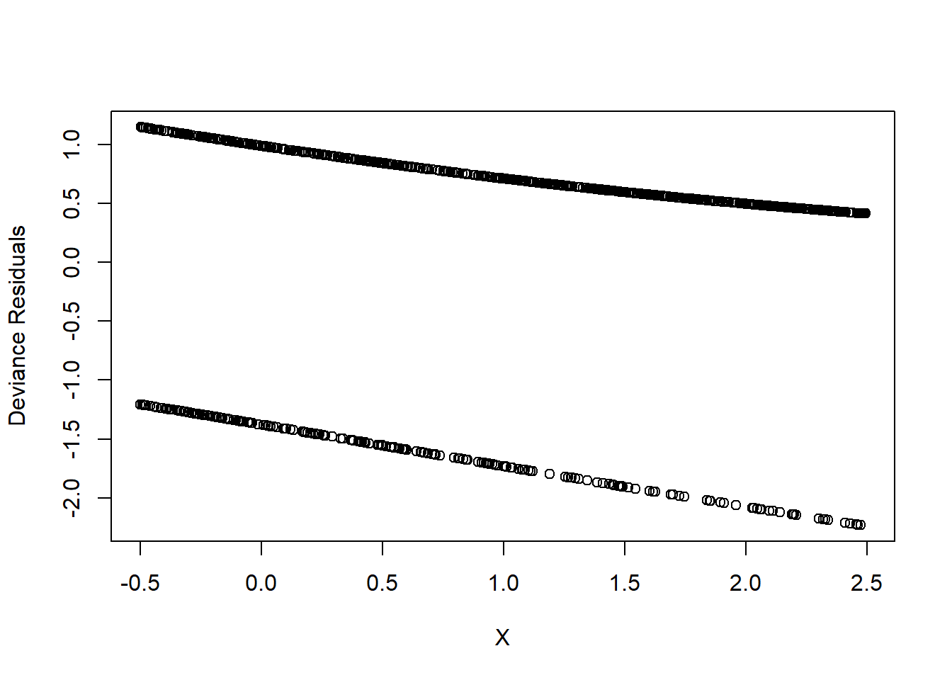
Figure 7.1: Deviance Residuals
This plot is not very informative. A more insightful approach is binned residual plots.
6. Binned Residual Plot
We group residuals into bins based on predicted values.
plot_bin <- function(Y,
                     X,
                     bins = 100,
                     return.DF = FALSE) {
  Y_Name <- deparse(substitute(Y))
  X_Name <- deparse(substitute(X))

  Binned_Plot <- data.frame(Plot_Y = Y, Plot_X = X)
  Binned_Plot$bin <-
    cut(Binned_Plot$Plot_X, breaks = bins) %>% as.numeric

  Binned_Plot_summary <- Binned_Plot %>%
    group_by(bin) %>%
    summarise(
      Y_ave = mean(Plot_Y),
      X_ave = mean(Plot_X),
      Count = n()
    ) %>% as.data.frame

  plot(
    y = Binned_Plot_summary$Y_ave,
    x = Binned_Plot_summary$X_ave,
    ylab = Y_Name,
    xlab = X_Name
  )

  if (return.DF)
    return(Binned_Plot_summary)
}

plot_bin(Y = Logistic_Resids, X = BinData$X, bins = 100)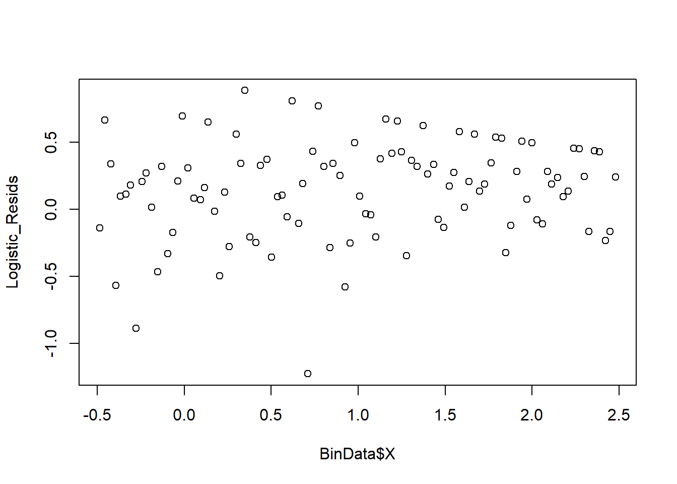
Figure 7.2: Binned Residual Plot
We also examine predicted values vs residuals:
Logistic_Predictions <- predict(Logistic_Model, type = "response")
plot_bin(Y = Logistic_Resids, X = Logistic_Predictions, bins = 100)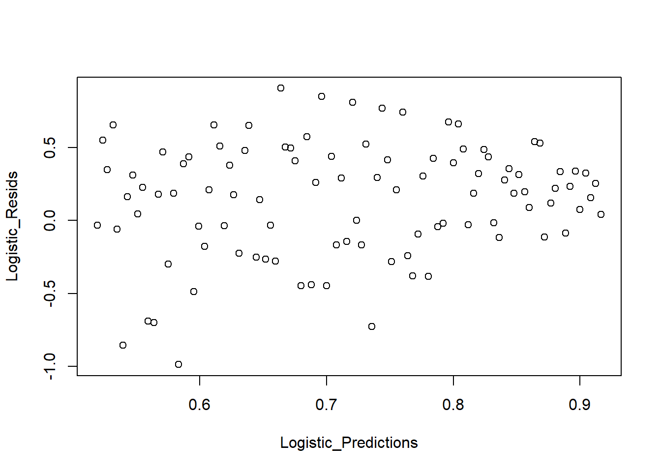
Figure 7.3: Predicted Values versus Residuals
Finally, we compare predicted probabilities to actual outcomes:
NumBins <- 10
Binned_Data <- plot_bin(
    Y = BinData$Y,
    X = Logistic_Predictions,
    bins = NumBins,
    return.DF = TRUE
)
Binned_Data
#>    bin     Y_ave     X_ave Count
#> 1    1 0.5833333 0.5382095    72
#> 2    2 0.5200000 0.5795887    75
#> 3    3 0.6567164 0.6156540    67
#> 4    4 0.7014925 0.6579674    67
#> 5    5 0.6373626 0.6984765    91
#> 6    6 0.7500000 0.7373341    72
#> 7    7 0.7096774 0.7786747    93
#> 8    8 0.8503937 0.8203819   127
#> 9    9 0.8947368 0.8601232   133
#> 10  10 0.8916256 0.9004734   203
abline(0, 1, lty = 2, col = 'blue')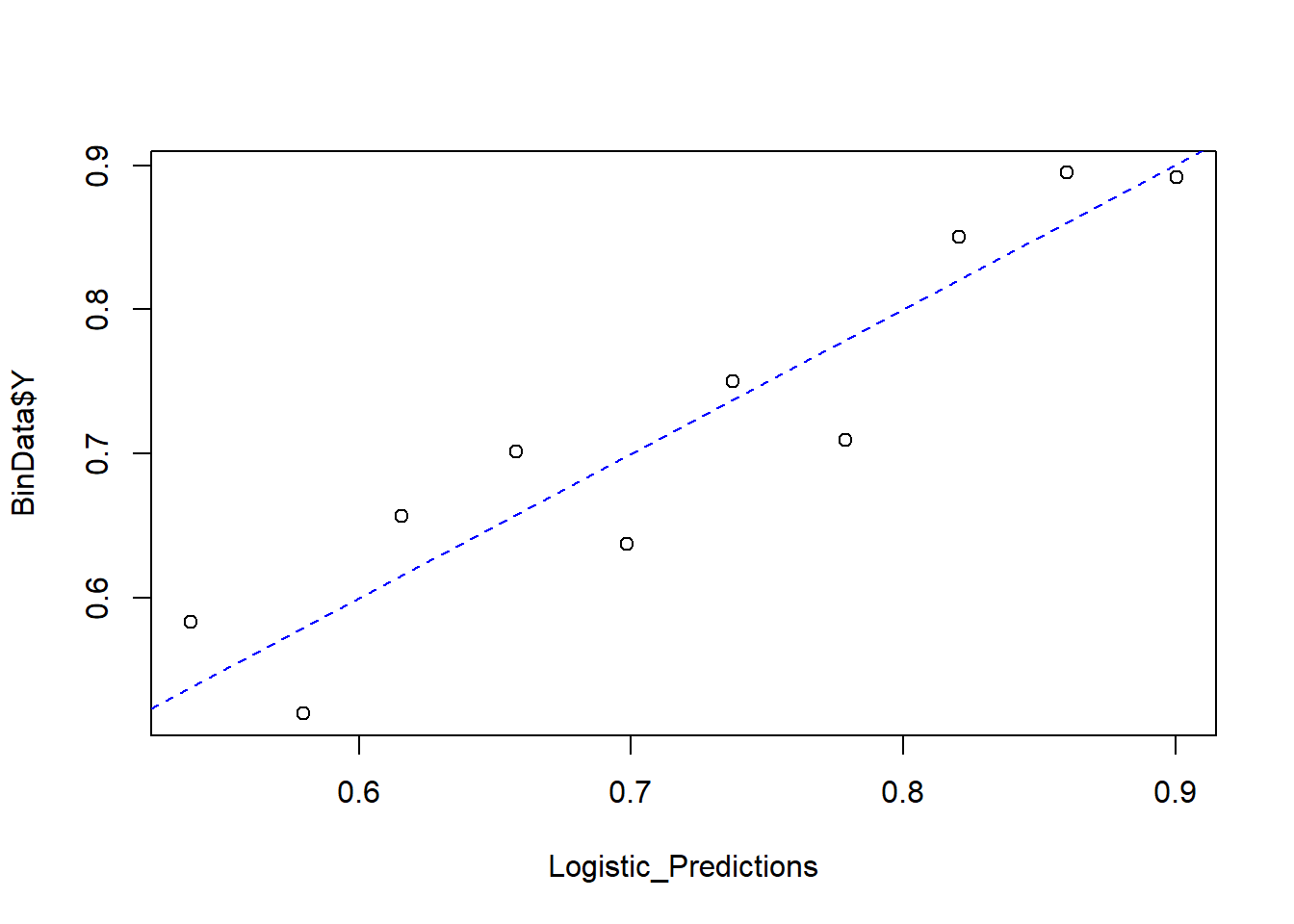
Figure 7.4: Predicted versus Actual Values
7. Model Goodness-of-Fit: Hosmer-Lemeshow Test
The Hosmer-Lemeshow test evaluates whether the model fits the data well. The test statistic is: \[ X^2_{HL} = \sum_{j=1}^{J} \frac{(y_j - m_j \hat{p}_j)^2}{m_j \hat{p}_j(1-\hat{p}_j)} \] where:
\(y_j\) is the observed number of successes in bin \(j\).
\(m_j\) is the number of observations in bin \(j\).
\(\hat{p}_j\) is the predicted probability in bin \(j\).
Under \(H_0\), we assume:
\[ X^2_{HL} \sim \chi^2_{J-1} \]
HL_BinVals <- (Binned_Data$Count * Binned_Data$Y_ave -
               Binned_Data$Count * Binned_Data$X_ave) ^ 2 /
               (Binned_Data$Count * Binned_Data$X_ave * (1 - Binned_Data$X_ave))

HLpval <- pchisq(q = sum(HL_BinVals),
                 df = NumBins - 1,
                 lower.tail = FALSE)
HLpval
#> [1] 0.4150004
Conclusion:
Since \(p\)-value = 0.99, we fail to reject \(H_0\).
This indicates that the model fits the data well.