39.2 Good Controls

39.2.1 Omitted Variable Bias Correction

A variable $Z$ is a good control when it blocks all back-door paths from the treatment $X$ to the outcome $Y$. This is the fundamental criterion from the back-door adjustment theorem in causal inference.

39.2.1.1 Simple Confounder

In this DAG, $Z$ is a common cause of both $X$ and $Y$, i.e., a confounder.

rm(list = ls())

model <- dagitty("dag{
  x -> y
  z -> x
  z -> y
}")
coordinates(model) <- list(
  x = c(x = 1, z = 2, y = 3),
  y = c(x = 1, z = 2, y = 1)
)
ggdag(model) + theme_dag()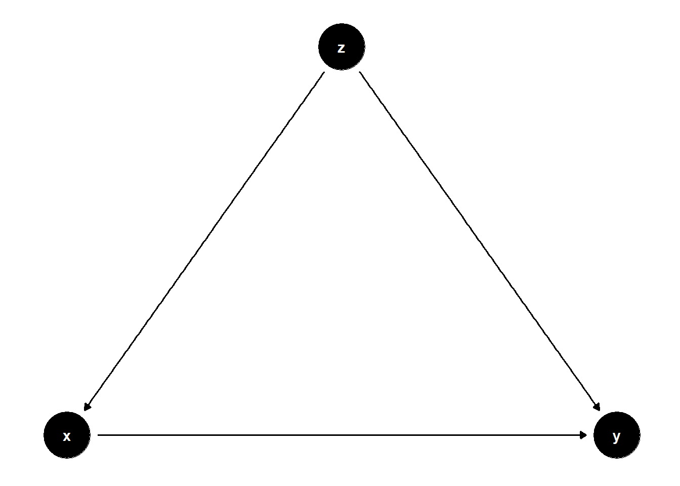

Controlling for $Z$ removes the bias from the back-door path $X \leftarrow Z \rightarrow Y$.

n <- 1e4
z <- rnorm(n)
causal_coef <- 2
beta2 <- 3
x <- z + rnorm(n)
y <- causal_coef * x + beta2 * z + rnorm(n)

jtools::export_summs(lm(y ~ x), lm(y ~ x + z))

	Model 1	Model 2
(Intercept)	-0.02	0.01
	(0.02)	(0.01)
x	3.49 ***	2.00 ***
	(0.02)	(0.01)
z		2.98 ***
		(0.01)
N	10000	10000
R2	0.82	0.97
*** p < 0.001; ** p < 0.01; * p < 0.05.

39.2.1.2 Confounding via a Latent Variable

In this structure, $U$ is unobserved but causes both $Z$ and $Y$, and $Z$ affects $X$. Even though $U$ is not observed, adjusting for $Z$ helps block the back-door path from $X$ to $Y$ that goes through $U$.

rm(list = ls())

model <- dagitty("dag{
  x -> y
  u -> z
  z -> x
  u -> y
}")
latents(model) <- "u"
coordinates(model) <- list(
  x = c(x = 1, z = 2, u = 3, y = 4),
  y = c(x = 1, z = 2, u = 3, y = 1)
)
ggdag(model) + theme_dag()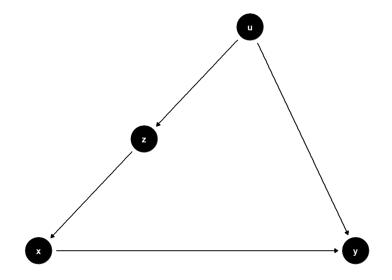

n <- 1e4
u <- rnorm(n)
z <- u + rnorm(n)
x <- z + rnorm(n)
y <- 2 * x + u + rnorm(n)

jtools::export_summs(lm(y ~ x), lm(y ~ x + z))

	Model 1	Model 2
(Intercept)	-0.02	-0.01
	(0.01)	(0.01)
x	2.33 ***	1.99 ***
	(0.01)	(0.01)
z		0.51 ***
		(0.01)
N	10000	10000
R2	0.91	0.92
*** p < 0.001; ** p < 0.01; * p < 0.05.

Even though $Z$ appears significant, its inclusion serves to reduce omitted variable bias rather than having a causal interpretation itself.

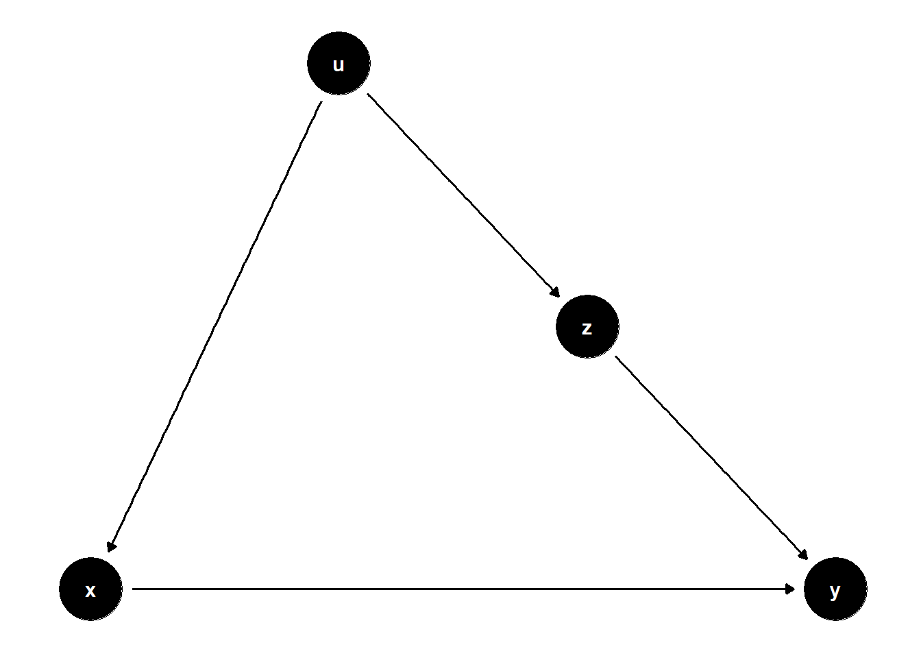
39.2.1.3 $Z$ is caused by $U$, but also causes $Y$

This DAG illustrates a subtle case where $Z$ is on a non-causal path from $X$ to $Y$ and helps block bias through a shared cause $U$.

rm(list = ls())

model <- dagitty("dag{
  x -> y
  u -> z
  u -> x
  z -> y
}")
latents(model) <- "u"
coordinates(model) <- list(
  x = c(x = 1, z = 3, u = 2, y = 4),
  y = c(x = 1, z = 2, u = 3, y = 1)
)
ggdag(model) + theme_dag()

n <- 1e4
u <- rnorm(n)
z <- u + rnorm(n)
x <- u + rnorm(n)
y <- 2 * x + z + rnorm(n)

jtools::export_summs(lm(y ~ x), lm(y ~ x + z))

	Model 1	Model 2
(Intercept)	0.02	0.01
	(0.02)	(0.01)
x	2.49 ***	1.98 ***
	(0.01)	(0.01)
z		1.02 ***
		(0.01)
N	10000	10000
R2	0.83	0.93
*** p < 0.001; ** p < 0.01; * p < 0.05.

Again, we cannot interpret the coefficient on $Z$ causally, but including $Z$ helps reduce omitted variable bias from the unobserved confounder $U$.

39.2.1.4 Summary of Omitted Variable Correction

# Model 1: Z is a confounder
model1 <- dagitty("dag{
  x -> y
  z -> x
  z -> y
}")
coordinates(model1) <-
    list(x = c(x = 1, z = 2, y = 3), y = c(x = 1, z = 2, y = 1))

# Model 2: Z is on path from U to X
model2 <- dagitty("dag{
  x -> y
  u -> z
  z -> x
  u -> y
}")
latents(model2) <- "u"
coordinates(model2) <-
    list(x = c(
        x = 1,
        z = 2,
        u = 3,
        y = 4
    ),
    y = c(
        x = 1,
        z = 2,
        u = 3,
        y = 1
    ))

# Model 3: Z influenced by U, affects Y
model3 <- dagitty("dag{
  x -> y
  u -> z
  u -> x
  z -> y
}")
latents(model3) <- "u"
coordinates(model3) <-
    list(x = c(
        x = 1,
        z = 3,
        u = 2,
        y = 4
    ),
    y = c(
        x = 1,
        z = 2,
        u = 3,
        y = 1
    ))

par(mfrow = c(1, 3))
ggdag(model1) + theme_dag()

ggdag(model2) + theme_dag()

ggdag(model3) + theme_dag()

39.2.2 Omitted Variable Bias in Mediation Correction

When a variable $Z$ is a confounder of both the treatment $X$ and a mediator $M$, controlling for $Z$ helps isolate the indirect and direct effects more accurately.

39.2.2.1 Observed Confounder of Mediator and Treatment

rm(list = ls())

model <- dagitty("dag{
  x -> y
  z -> x
  x -> m
  z -> m
  m -> y
}")
coordinates(model) <-
    list(x = c(
        x = 1,
        z = 2,
        m = 3,
        y = 4
    ),
    y = c(
        x = 1,
        z = 2,
        m = 1,
        y = 1
    ))
ggdag(model) + theme_dag()

n <- 1e4
z <- rnorm(n)
x <- z + rnorm(n)
m <- 2 * x + z + rnorm(n)
y <- m + rnorm(n)

jtools::export_summs(lm(y ~ x), lm(y ~ x + z))

	Model 1	Model 2
(Intercept)	-0.01	0.01
	(0.02)	(0.01)
x	2.50 ***	1.99 ***
	(0.01)	(0.01)
z		1.01 ***
		(0.02)
N	10000	10000
R2	0.84	0.87
*** p < 0.001; ** p < 0.01; * p < 0.05.

39.2.2.2 Latent Common Cause of Mediator and Treatment

rm(list = ls())

model <- dagitty("dag{
  x -> y
  u -> z
  z -> x
  x -> m
  u -> m
  m -> y
}")
latents(model) <- "u"
coordinates(model) <-
    list(x = c(
        x = 1,
        z = 2,
        u = 3,
        m = 4,
        y = 5
    ),
    y = c(
        x = 1,
        z = 2,
        u = 3,
        m = 1,
        y = 1
    ))
ggdag(model) + theme_dag()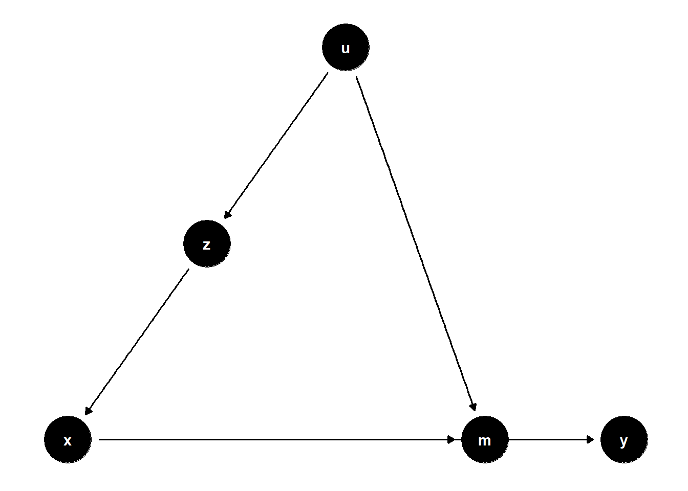

n <- 1e4
u <- rnorm(n)
z <- u + rnorm(n)
x <- z + rnorm(n)
m <- 2 * x + u + rnorm(n)
y <- m + rnorm(n)

jtools::export_summs(lm(y ~ x), lm(y ~ x + z))

	Model 1	Model 2
(Intercept)	0.01	0.01
	(0.02)	(0.02)
x	2.34 ***	2.01 ***
	(0.01)	(0.02)
z		0.50 ***
		(0.02)
N	10000	10000
R2	0.86	0.87
*** p < 0.001; ** p < 0.01; * p < 0.05.

39.2.2.3 Z Affects Mediator, U Affects Both X and Z

rm(list = ls())

model <- dagitty("dag{
  x -> y
  u -> z
  z -> m
  x -> m
  u -> x
  m -> y
}")
latents(model) <- "u"
coordinates(model) <-
    list(x = c(
        x = 1,
        z = 3,
        u = 2,
        m = 4,
        y = 5
    ),
    y = c(
        x = 1,
        z = 2,
        u = 3,
        m = 1,
        y = 1
    ))
ggdag(model) + theme_dag()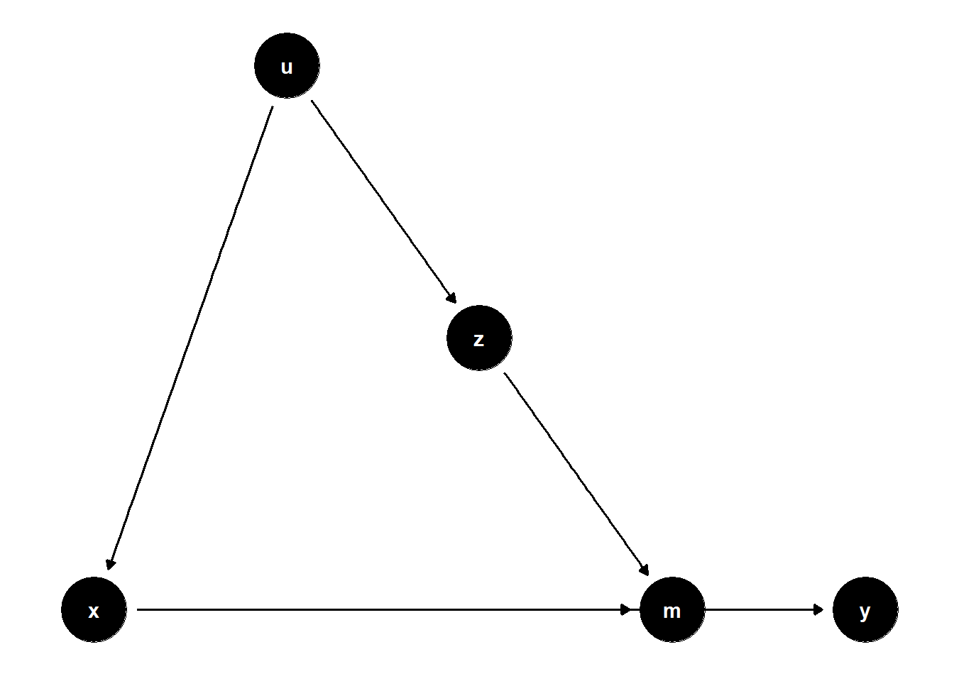

n <- 1e4
u <- rnorm(n)
z <- u + rnorm(n)
x <- u + rnorm(n)
m <- 2 * x + z + rnorm(n)
y <- m + rnorm(n)

jtools::export_summs(lm(y ~ x), lm(y ~ x + z))

	Model 1	Model 2
(Intercept)	0.00	0.00
	(0.02)	(0.01)
x	2.49 ***	1.99 ***
	(0.01)	(0.01)
z		1.00 ***
		(0.01)
N	10000	10000
R2	0.78	0.87
*** p < 0.001; ** p < 0.01; * p < 0.05.

39.2.2.4 Summary of Mediation Correction

# Model 4
model4 <- dagitty("dag{
  x -> y
  z -> x
  x -> m
  z -> m
  m -> y
}")
coordinates(model4) <-
    list(x = c(
        x = 1,
        z = 2,
        m = 3,
        y = 4
    ),
    y = c(
        x = 1,
        z = 2,
        m = 1,
        y = 1
    ))

# Model 5
model5 <- dagitty("dag{
  x -> y
  u -> z
  z -> x
  x -> m
  u -> m
  m -> y
}")
latents(model5) <- "u"
coordinates(model5) <-
    list(x = c(
        x = 1,
        z = 2,
        u = 3,
        m = 4,
        y = 5
    ),
    y = c(
        x = 1,
        z = 2,
        u = 3,
        m = 1,
        y = 1
    ))

# Model 6
model6 <- dagitty("dag{
  x -> y
  u -> z
  z -> m
  x -> m
  u -> x
  m -> y
}")
latents(model6) <- "u"
coordinates(model6) <-
    list(x = c(
        x = 1,
        z = 3,
        u = 2,
        m = 4,
        y = 5
    ),
    y = c(
        x = 1,
        z = 2,
        u = 3,
        m = 1,
        y = 1
    ))

par(mfrow = c(1, 3))
ggdag(model4) + theme_dag()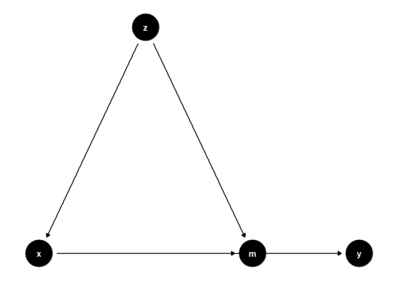

ggdag(model5) + theme_dag()

ggdag(model6) + theme_dag()

While $Z$ may be statistically significant, this does not imply a causal effect unless $Z$ is directly on the causal path from $X$ to $Y$. In many valid control scenarios, $Z$ simply serves to isolate the causal effect of $X$, not to be interpreted as a cause itself.

---