10.7 Generalized Additive Models
A generalized additive model (GAM) extends generalized linear models by allowing additive smooth terms:
\[ g(\mathbb{E}[Y]) = \beta_0 + f_1(X_1) + f_2(X_2) + \cdots + f_p(X_p), \]
where:
- \(g(\cdot)\) is a link function (as in GLMs),
- \(\beta_0\) is the intercept,
- Each \(f_j\) is a smooth, potentially nonparametric function (e.g., a spline, kernel smoother, or local polynomial smoother),
- \(p\) is the number of predictors, with \(p \ge 2\) highlighting the flexibility of GAMs in handling multivariate data.
This structure allows for nonlinear relationships between each predictor \(X_j\) and the response \(Y\), while maintaining additivity, which simplifies interpretation compared to fully nonparametric models.
Traditional linear models assume a strictly linear relationship:
\[ g(\mathbb{E}[Y]) = \beta_0 + \beta_1 X_1 + \beta_2 X_2 + \cdots + \beta_p X_p. \]
However, real-world data often exhibit complex, nonlinear patterns. While generalized linear models extend linear models to non-Gaussian responses, they still rely on linear predictors. GAMs address this by replacing linear terms with smooth functions:
- GLMs: Linear effects (e.g., \(\beta_1 X_1\))
- GAMs: Nonlinear smooth effects (e.g., \(f_1(X_1)\))
The general form of a GAM is:
\[ g(\mathbb{E}[Y \mid \mathbf{X}]) = \beta_0 + \sum_{j=1}^p f_j(X_j), \]
where:
- \(Y\) is the response variable,
- \(\mathbf{X} = (X_1, X_2, \ldots, X_p)\) are the predictors,
- \(f_j\) are smooth functions capturing potentially nonlinear effects,
- The link function \(g(\cdot)\) connects the mean of \(Y\) to the additive predictor.
Special Cases:
- When \(g\) is the identity function and \(Y\) is continuous: This reduces to an additive model (a special case of GAM).
- When \(g\) is the logit function and \(Y\) is binary: We have a logistic GAM for classification tasks.
- When \(g\) is the log function and \(Y\) follows a Poisson distribution: This is a Poisson GAM for count data.
10.7.1 Estimation via Penalized Likelihood
GAMs are typically estimated using penalized likelihood methods to balance model fit and smoothness. The objective function is:
\[ \mathcal{L}_{\text{pen}} = \ell(\beta_0, f_1, \ldots, f_p) - \frac{1}{2} \sum_{j=1}^p \lambda_j \int \left(f_j''(x)\right)^2 dx, \]
where:
- \(\ell(\beta_0, f_1, \ldots, f_p)\) is the (log-)likelihood of the data,
- \(\lambda_j \ge 0\) are smoothing parameters controlling the smoothness of each \(f_j\),
- The penalty term \(\int (f_j'')^2 dx\) discourages excessive curvature, similar to smoothing splines.
10.7.1.1 Backfitting Algorithm
For continuous responses, the classic backfitting algorithm is often used:
- Initialize: Start with an initial guess for each \(f_j\), typically zero.
- Iterate: For each \(j = 1, \dots, p\):
- Compute the partial residuals: \[ r_j = y - \beta_0 - \sum_{k \neq j} f_k(X_k) \]
- Update \(f_j\) by fitting a smoother to \((X_j, r_j)\).
- Convergence: Repeat until the functions \(f_j\) stabilize.
This approach works because of the additive structure, which allows each smooth term to be updated conditionally on the others.
10.7.1.2 Generalized Additive Model Estimation (for GLMs)
When \(Y\) is non-Gaussian (e.g., binary, count data), we use iteratively reweighted least squares (IRLS) in combination with backfitting. Popular implementations, such as in the mgcv package in R, use penalized likelihood estimation with efficient computational algorithms (e.g., penalized iteratively reweighted least squares).
10.7.2 Interpretation of GAMs
One of the key advantages of GAMs is their interpretability, especially compared to fully nonparametric or black-box machine learning models.
- Additive Structure: Each predictor’s effect is modeled separately via \(f_j(X_j)\), making it easy to interpret marginal effects.
- Partial Dependence Plots: Visualization of \(f_j(X_j)\) shows how each predictor affects the response, holding other variables constant.
Example:
For a marketing dataset predicting customer purchase probability:
\[ \log\left(\frac{\mathbb{P}(\text{Purchase})}{1 - \mathbb{P}(\text{Purchase})}\right) = \beta_0 + f_1(\text{Age}) + f_2(\text{Income}) + f_3(\text{Ad Exposure}) \]
- \(f_1(\text{Age})\) might show a peak in purchase likelihood for middle-aged customers.
- \(f_2(\text{Income})\) could reveal a threshold effect where purchases increase beyond a certain income level.
- \(f_3(\text{Ad Exposure})\) might show diminishing returns after repeated exposures.
10.7.3 Model Selection and Smoothing Parameter Estimation
The smoothing parameters \(\lambda_j\) control the complexity of each smooth term:
- Large \(\lambda_j\): Strong smoothing, leading to nearly linear fits.
- Small \(\lambda_j\): Flexible, wiggly fits that may overfit if \(\lambda_j\) is too small.
Methods for Choosing \(\lambda_j\):
Generalized Cross-Validation (GCV): \[ \mathrm{GCV} = \frac{1}{n} \frac{\sum_{i=1}^n (y_i - \hat{y}_i)^2}{\left(1 - \frac{\operatorname{tr}(\mathbf{S})}{n}\right)^2} \] where \(\mathbf{S}\) is the smoother matrix. GCV is a popular method for selecting the smoothing parameter \(\lambda_j\) because it approximates leave-one-out cross-validation without requiring explicit refitting of the model. The term \(\text{tr}(\mathbf{S})\) represents the effective degrees of freedom of the smoother, and the denominator penalizes overfitting.
Unbiased Risk Estimation: This method extends the idea of GCV to non-Gaussian families (e.g., Poisson, binomial). It aims to minimize an unbiased estimate of the risk (expected prediction error). For Gaussian models, it often reduces to a form similar to GCV, but for other distributions, it incorporates the appropriate likelihood or deviance.
Akaike Information Criterion (AIC): \[ AIC=−2\log(L)+2tr(S) \] where \(L\) is the likelihood of the model. AIC balances model fit (measured by the likelihood) and complexity (measured by the effective degrees of freedom \(tr(S)\)). The smoothing parameter \(\lambda_j\) is chosen to minimize the AIC.
Bayesian Information Criterion (BIC): \[ BIC=−2\log(L)+\log(n)tr(S) \] where \(n\) is the sample size. BIC is similar to AIC but imposes a stronger penalty for model complexity, making it more suitable for larger datasets.
Leave-One-Out Cross-Validation (LOOCV): \[ LOOCV = \frac{1}{n}\sum_{i = 1}^n ( y_i - \hat{y}_i^{(-i)})^2, \] where \(y_i^{(−i)}\) is the predicted value for the ii-th observation when the model is fitted without it. LOOCV is computationally intensive but provides a direct estimate of prediction error.
Empirical Risk Minimization:
For some non-parametric regression methods, \(\lambda_j\) can be chosen by minimizing the empirical risk (e.g., mean squared error) on a validation set or via resampling techniques like \(k\)-fold cross-validation.
10.7.4 Extensions of GAMs
GAM with Interaction Terms: \[ g(\mathbb{E}[Y]) = \beta_0 + f_1(X_1) + f_2(X_2) + f_{12}(X_1, X_2) \] where \(f_{12}\) captures the interaction between \(X_1\) and \(X_2\) (using tensor product smooths).
GAMMs (Generalized Additive Mixed Models): Incorporate random effects to handle hierarchical or grouped data.
Varying Coefficient Models: Allow regression coefficients to vary smoothly with another variable, e.g., \[ Y = \beta_0 + f_1(Z) \cdot X + \varepsilon \]
# Load necessary libraries
library(mgcv)    # For fitting GAMs
library(ggplot2)
library(gridExtra)

# Simulate Data
set.seed(123)

n <- 100
x1 <- runif(n, 0, 10)
x2 <- runif(n, 0, 5)
x3 <- rnorm(n, 5, 2)

# True nonlinear functions
f1 <- function(x)
    sin(x)                 # Nonlinear effect of x1
f2 <- function(x)
    log(x + 1)             # Nonlinear effect of x2
f3 <- function(x)
    0.5 * (x - 5) ^ 2        # Quadratic effect for x3

# Generate response variable with noise
y <- 3 + f1(x1) + f2(x2) - f3(x3) + rnorm(n, sd = 1)

# Data frame for analysis
data_gam <- data.frame(y, x1, x2, x3)

# Plotting the true functions with simulated data
p1 <-
    ggplot(data_gam, aes(x1, y)) +
    geom_point() +
    labs(title = "Effect of x1 (sin(x1))")
p2 <-
    ggplot(data_gam, aes(x2, y)) +
    geom_point() +
    labs(title = "Effect of x2 (log(x2+1))")
p3 <-
    ggplot(data_gam, aes(x3, y)) +
    geom_point() +
    labs(title = "Effect of x3 (quadratic)")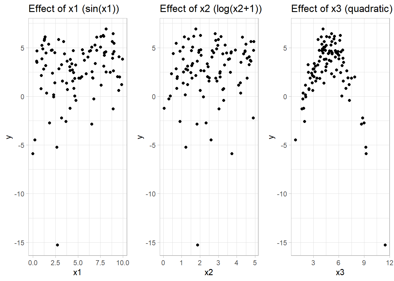
Figure 10.15: Scatter Plot Effect of X
# Fit a GAM using mgcv
gam_model <-
    gam(y ~ s(x1) + s(x2) + s(x3),
        data = data_gam, method = "REML")

# Summary of the model
summary(gam_model)
#>
#> Family: gaussian
#> Link function: identity
#>
#> Formula:
#> y ~ s(x1) + s(x2) + s(x3)
#>
#> Parametric coefficients:
#>             Estimate Std. Error t value Pr(>|t|)
#> (Intercept)  2.63937    0.09511   27.75   <2e-16 ***
#> ---
#> Signif. codes:  0 '***' 0.001 '**' 0.01 '*' 0.05 '.' 0.1 ' ' 1
#>
#> Approximate significance of smooth terms:
#>         edf Ref.df       F p-value
#> s(x1) 5.997  7.165   7.966   5e-07 ***
#> s(x2) 1.000  1.000  10.249 0.00192 **
#> s(x3) 6.239  7.343 105.551 < 2e-16 ***
#> ---
#> Signif. codes:  0 '***' 0.001 '**' 0.01 '*' 0.05 '.' 0.1 ' ' 1
#>
#> R-sq.(adj) =   0.91   Deviance explained = 92.2%
#> -REML = 155.23  Scale est. = 0.90463   n = 100
# Plot smooth terms
par(mfrow = c(1, 3)) # Arrange plots in one row
plot(gam_model, shade = TRUE, seWithMean = TRUE)-1.png)
(#fig:Visualizing Smooth Functions (Partial Dependence Plots))Smooth Functions
# Using ggplot2 with mgcv's predict function
pred_data <- with(data_gam, expand.grid(
    x1 = seq(min(x1), max(x1), length.out = 100),
    x2 = mean(x2),
    x3 = mean(x3)
))

# Predictions for x1 effect
pred_data$pred_x1 <-
predict(gam_model, newdata = pred_data, type = "response")ggplot(pred_data, aes(x1, pred_x1)) +
geom_line(color = "blue", size = 1.2) +
labs(title = "Partial Effect of x1",
x = "x1",
y = "Effect on y") +
theme_minimal()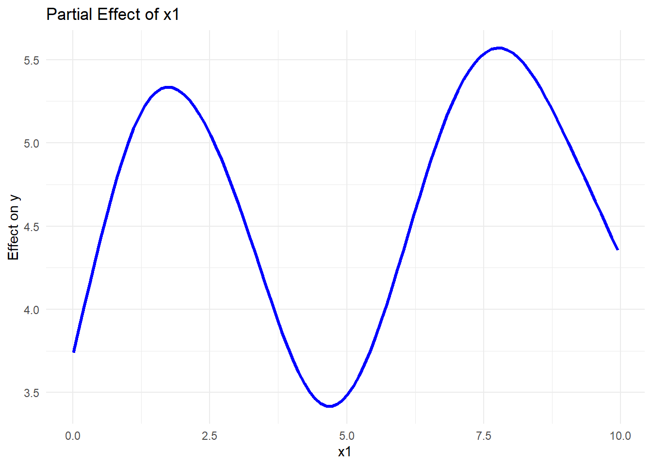
Figure 10.16: Partial Effect of x1
# Check AIC and GCV score
AIC(gam_model)
#> [1] 289.8201
gam_model$gcv.ubre  # GCV/UBRE score
#>     REML
#> 155.2314
#> attr(,"Dp")
#> [1] 47.99998


# Compare models with different smoothness
gam_model_simple <-
    gam(y ~ s(x1, k = 4) + s(x2, k = 4) + s(x3, k = 4),
        data = data_gam)
gam_model_complex <-
    gam(y ~ s(x1, k = 20) + s(x2, k = 20) + s(x3, k = 20),
        data = data_gam)

# Compare models using AIC
AIC(gam_model, gam_model_simple, gam_model_complex)
#>                          df      AIC
#> gam_model         15.706428 289.8201
#> gam_model_simple   8.429889 322.1502
#> gam_model_complex 13.571165 287.4171- Lower AIC indicates a better model balancing fit and complexity.
- GCV score helps select the optimal level of smoothness.
- Compare models to prevent overfitting (too flexible) or underfitting (too simple).
# GAM with interaction using tensor product smooths
gam_interaction <- gam(y ~ te(x1, x2) + s(x3),
                       data = data_gam)

# Summary of the interaction model
summary(gam_interaction)
#>
#> Family: gaussian
#> Link function: identity
#>
#> Formula:
#> y ~ te(x1, x2) + s(x3)
#>
#> Parametric coefficients:
#>             Estimate Std. Error t value Pr(>|t|)
#> (Intercept)  2.63937    0.09364   28.19   <2e-16 ***
#> ---
#> Signif. codes:  0 '***' 0.001 '**' 0.01 '*' 0.05 '.' 0.1 ' ' 1
#>
#> Approximate significance of smooth terms:
#>             edf Ref.df       F p-value
#> te(x1,x2) 8.545  8.923   9.218  <2e-16 ***
#> s(x3)     4.766  5.834 147.595  <2e-16 ***
#> ---
#> Signif. codes:  0 '***' 0.001 '**' 0.01 '*' 0.05 '.' 0.1 ' ' 1
#>
#> R-sq.(adj) =  0.912   Deviance explained = 92.4%
#> GCV = 1.0233  Scale est. = 0.87688   n = 100
# Visualization of interaction effect
vis.gam(
gam_interaction,
view = c("x1", "x2"),
plot.type = "contour",
color = "terrain"
)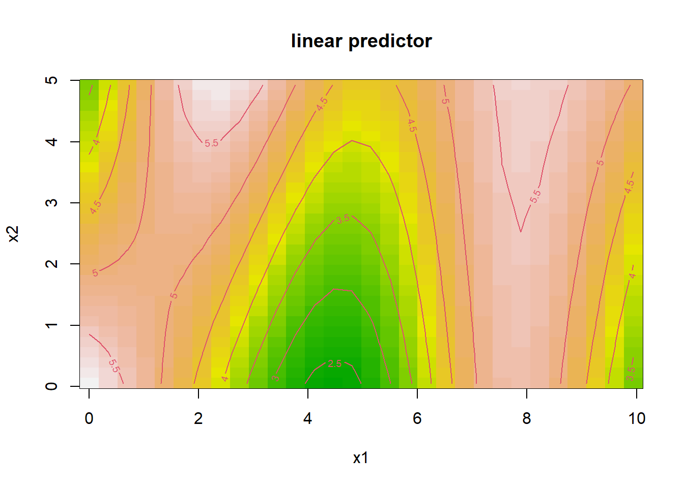
Figure 10.17: Linear Predictor
- The tensor product smooth
te(x1, x2)captures nonlinear interactions betweenx1andx2. - The contour plot visualizes how their joint effect influences the response.
# Simulate binary response
set.seed(123)
prob <- plogis(1 + f1(x1) - f2(x2) + 0.3 * x3)  # Logistic function
y_bin <- rbinom(n, 1, prob)                     # Binary outcome

# Fit GAM for binary classification
gam_logistic <-
    gam(y_bin ~ s(x1) + s(x2) + s(x3),
        family = binomial,
        data = data_gam)

# Summary and visualization
summary(gam_logistic)
#>
#> Family: binomial
#> Link function: logit
#>
#> Formula:
#> y_bin ~ s(x1) + s(x2) + s(x3)
#>
#> Parametric coefficients:
#>             Estimate Std. Error z value Pr(>|z|)
#> (Intercept)    22.30      32.18   0.693    0.488
#>
#> Approximate significance of smooth terms:
#>         edf Ref.df Chi.sq p-value
#> s(x1) 4.472  5.313  2.645   0.775
#> s(x2) 1.000  1.000  1.925   0.165
#> s(x3) 1.000  1.000  1.390   0.238
#>
#> R-sq.(adj) =      1   Deviance explained = 99.8%
#> UBRE = -0.84802  Scale est. = 1         n = 100
Figure 2.5: Smooth Functions of Variables
- The logistic GAM models nonlinear effects on the log-odds of the binary outcome.
- Smooth plots indicate predictors’ influence on probability of success.
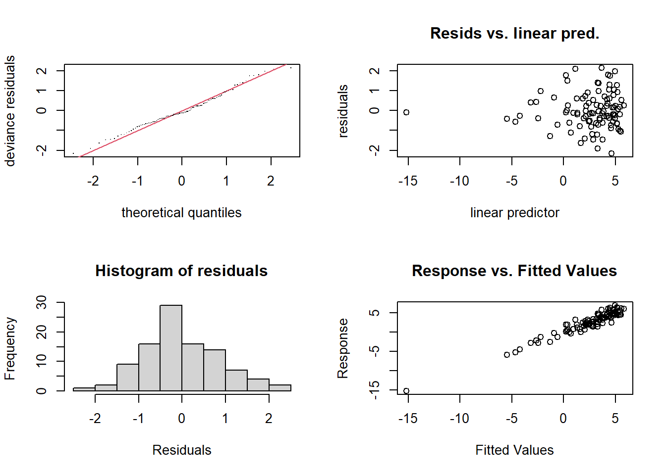
(#fig:Model Diagnostics)Model Diagnostics
#>
#> Method: REML   Optimizer: outer newton
#> full convergence after 9 iterations.
#> Gradient range [-5.387854e-05,2.006026e-05]
#> (score 155.2314 & scale 0.9046299).
#> Hessian positive definite, eigenvalue range [5.387409e-05,48.28647].
#> Model rank =  28 / 28
#>
#> Basis dimension (k) checking results. Low p-value (k-index<1) may
#> indicate that k is too low, especially if edf is close to k'.
#>
#>         k'  edf k-index p-value
#> s(x1) 9.00 6.00    1.01    0.46
#> s(x2) 9.00 1.00    1.16    0.92
#> s(x3) 9.00 6.24    1.07    0.72
par(mfrow = c(1, 1))- Residual plots assess model fit.
- QQ plot checks for normality of residuals.
- K-index evaluates the adequacy of smoothness selection.