7.7 Multinomial Logistic Regression
When dealing with categorical response variables with more than two possible outcomes, the multinomial logistic regression is a natural extension of the binary logistic model.
7.7.1 The Multinomial Distribution
Suppose we have a categorical response variable \(Y_i\) that can take values in \(\{1, 2, \dots, J\}\). For each observation \(i\), the probability that it falls into category \(j\) is given by:
\[ p_{ij} = P(Y_i = j), \quad \text{where} \quad \sum_{j=1}^{J} p_{ij} = 1. \]
The response follows a multinomial distribution:
\[ Y_i \sim \text{Multinomial}(1; p_{i1}, p_{i2}, ..., p_{iJ}). \]
This means that each observation belongs to exactly one of the \(J\) categories.
7.7.2 Modeling Probabilities Using Log-Odds
We cannot model the probabilities \(p_{ij}\) directly because they must sum to 1. Instead, we use a logit transformation, comparing each category \(j\) to a baseline category (typically the first category, \(j=1\)):
\[ \eta_{ij} = \log \frac{p_{ij}}{p_{i1}}, \quad j = 2, \dots, J. \]
Using a linear function of covariates \(\mathbf{x}_i\), we define:
\[ \eta_{ij} = \mathbf{x}_i' \beta_j = \beta_{j0} + \sum_{p=1}^{P} \beta_{jp} x_{ip}. \]
Rearranging to express probabilities explicitly:
\[ p_{ij} = p_{i1} \exp(\mathbf{x}_i' \beta_j). \]
Since all probabilities must sum to 1:
\[ p_{i1} + \sum_{j=2}^{J} p_{ij} = 1. \]
Substituting for \(p_{ij}\):
\[ p_{i1} + \sum_{j=2}^{J} p_{i1} \exp(\mathbf{x}_i' \beta_j) = 1. \]
Solving for \(p_{i1}\):
\[ p_{i1} = \frac{1}{1 + \sum_{j=2}^{J} \exp(\mathbf{x}_i' \beta_j)}. \]
Thus, the probability for category \(j\) is:
\[ p_{ij} = \frac{\exp(\mathbf{x}_i' \beta_j)}{1 + \sum_{l=2}^{J} \exp(\mathbf{x}_i' \beta_l)}, \quad j = 2, \dots, J. \]
This formulation is known as the multinomial logit model.
7.7.3 Softmax Representation
An alternative formulation avoids choosing a baseline category and instead treats all \(J\) categories symmetrically using the softmax function:
\[ P(Y_i = j | X_i = x) = \frac{\exp(\beta_{j0} + \sum_{p=1}^{P} \beta_{jp} x_p)}{\sum_{l=1}^{J} \exp(\beta_{l0} + \sum_{p=1}^{P} \beta_{lp} x_p)}. \]
This representation is often used in neural networks and general machine learning models.
7.7.4 Log-Odds Ratio Between Two Categories
The log-odds ratio between two categories \(k\) and \(k'\) is:
\[ \log \frac{P(Y = k | X = x)}{P(Y = k' | X = x)} = (\beta_{k0} - \beta_{k'0}) + \sum_{p=1}^{P} (\beta_{kp} - \beta_{k'p}) x_p. \]
This equation tells us that:
- If \(\beta_{kp} > \beta_{k'p}\), then increasing \(x_p\) increases the odds of choosing category \(k\) over \(k'\).
- If \(\beta_{kp} < \beta_{k'p}\), then increasing \(x_p\) decreases the odds of choosing \(k\) over \(k'\).
7.7.5 Estimation
To estimate the parameters \(\beta_j\), we use Maximum Likelihood estimation.
Given \(n\) independent observations \((Y_i, X_i)\), the likelihood function is:
\[ L(\beta) = \prod_{i=1}^{n} \prod_{j=1}^{J} p_{ij}^{Y_{ij}}. \]
Taking the log-likelihood:
\[ \log L(\beta) = \sum_{i=1}^{n} \sum_{j=1}^{J} Y_{ij} \log p_{ij}. \]
Since there is no closed-form solution, numerical methods (see Non-linear Least Squares Estimation) are used for estimation.
7.7.6 Interpretation of Coefficients
- Each \(\beta_{jp}\) represents the effect of \(x_p\) on the log-odds of category \(j\) relative to the baseline.
- Positive coefficients mean increasing \(x_p\) makes category \(j\) more likely relative to the baseline.
- Negative coefficients mean increasing \(x_p\) makes category \(j\) less likely relative to the baseline.
7.7.7 Application: Multinomial Logistic Regression
1. Load Necessary Libraries and Data
library(faraway)  # For the dataset
library(dplyr)    # For data manipulation
library(ggplot2)  # For visualization
library(nnet)     # For multinomial logistic regression

# Load and inspect data
data(nes96, package="faraway")
head(nes96, 3)
#>   popul TVnews selfLR ClinLR DoleLR     PID age  educ   income    vote
#> 1     0      7 extCon extLib    Con  strRep  36    HS $3Kminus    Dole
#> 2   190      1 sliLib sliLib sliCon weakDem  20  Coll $3Kminus Clinton
#> 3    31      7    Lib    Lib    Con weakDem  24 BAdeg $3Kminus Clinton
The dataset nes96 contains survey responses, including political party identification (PID), age (age), and education level (educ).
2. Define Political Strength Categories
We classify political strength into three categories:
Strong: Strong Democrat or Strong Republican
Weak: Weak Democrat or Weak Republican
Neutral: Independents and other affiliations
# Check distribution of political identity
table(nes96$PID)
#>
#>  strDem weakDem  indDem  indind  indRep weakRep  strRep
#>     200     180     108      37      94     150     175

# Define Political Strength variable
nes96 <- nes96 %>%
  mutate(Political_Strength = case_when(
    PID %in% c("strDem", "strRep") ~ "Strong",
    PID %in% c("weakDem", "weakRep") ~ "Weak",
    PID %in% c("indDem", "indind", "indRep") ~ "Neutral",
    TRUE ~ NA_character_
  ))

# Summarize
nes96 %>% group_by(Political_Strength) %>% summarise(Count = n())
#> # A tibble: 3 × 2
#>   Political_Strength Count
#>   <chr>              <int>
#> 1 Neutral              239
#> 2 Strong               375
#> 3 Weak                 330
3. Visualizing Political Strength by Age
We visualize the proportion of each political strength category across age groups.
# Prepare data for visualization
Plot_DF <- nes96 %>%
    mutate(Age_Grp = cut_number(age, 4)) %>%
    group_by(Age_Grp, Political_Strength) %>%
    summarise(count = n(), .groups = 'drop') %>%
    group_by(Age_Grp) %>%
    mutate(etotal = sum(count), proportion = count / etotal)

# Plot age vs political strength
Age_Plot <- ggplot(
    Plot_DF,
    aes(
        x        = Age_Grp,
        y        = proportion,
        group    = Political_Strength,
        linetype = Political_Strength,
        color    = Political_Strength
    )
) +
    geom_line(size = 2) +
    labs(title = "Political Strength by Age Group",
         x = "Age Group",
         y = "Proportion")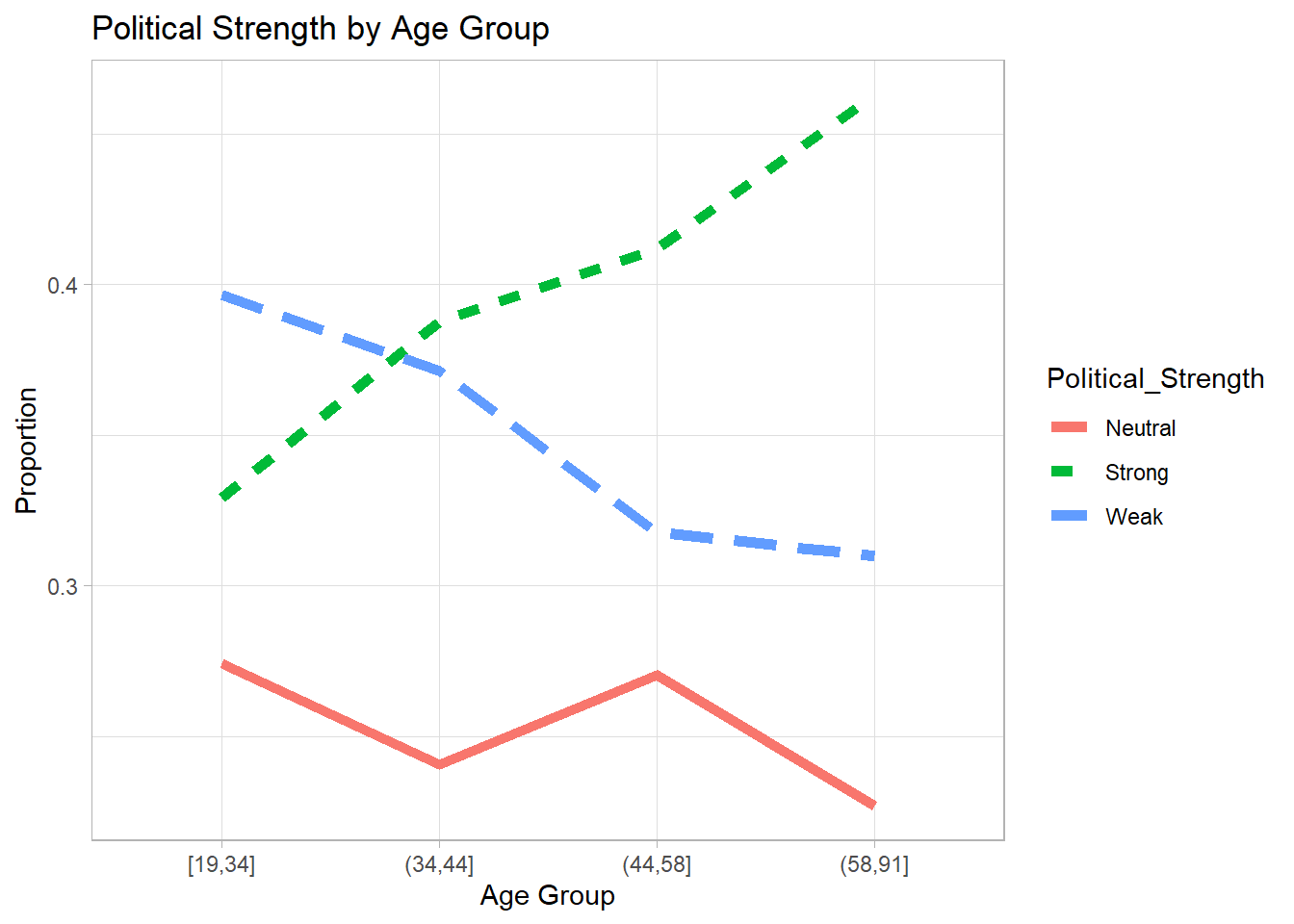
Figure 7.9: Political Strength by Age Group
4. Fit a Multinomial Logistic Model
We model political strength as a function of age and education.
# Fit multinomial logistic regression
Multinomial_Model <-
    multinom(Political_Strength ~ age + educ,
             data = nes96,
             trace = FALSE)
summary(Multinomial_Model)
#> Call:
#> multinom(formula = Political_Strength ~ age + educ, data = nes96,
#>     trace = FALSE)
#>
#> Coefficients:
#>        (Intercept)          age     educ.L     educ.Q     educ.C      educ^4
#> Strong -0.08788729  0.010700364 -0.1098951 -0.2016197 -0.1757739 -0.02116307
#> Weak    0.51976285 -0.004868771 -0.1431104 -0.2405395 -0.2411795  0.18353634
#>            educ^5     educ^6
#> Strong -0.1664377 -0.1359449
#> Weak   -0.1489030 -0.2173144
#>
#> Std. Errors:
#>        (Intercept)         age    educ.L    educ.Q    educ.C    educ^4
#> Strong   0.3017034 0.005280743 0.4586041 0.4318830 0.3628837 0.2964776
#> Weak     0.3097923 0.005537561 0.4920736 0.4616446 0.3881003 0.3169149
#>           educ^5    educ^6
#> Strong 0.2515012 0.2166774
#> Weak   0.2643747 0.2199186
#>
#> Residual Deviance: 2024.596
#> AIC: 2056.596
5. Stepwise Model Selection Based on AIC
We perform stepwise selection to find the best model.
Multinomial_Step <- step(Multinomial_Model, trace = 0)
#> trying - age
#> trying - educ
#> trying - age
Multinomial_Step
#> Call:
#> multinom(formula = Political_Strength ~ age, data = nes96, trace = FALSE)
#>
#> Coefficients:
#>        (Intercept)          age
#> Strong -0.01988977  0.009832916
#> Weak    0.59497046 -0.005954348
#>
#> Residual Deviance: 2030.756
#> AIC: 2038.756
Compare the best model to the full model based on deviance:
pchisq(
    q = deviance(Multinomial_Step) - deviance(Multinomial_Model),
    df = Multinomial_Model$edf - Multinomial_Step$edf,
    lower.tail = FALSE
)
#> [1] 0.9078172
A non-significant p-value suggests no major difference between the full and stepwise models.
6. Predictions & Visualization
Predicting Political Strength Probabilities by Age
# Create data for prediction
PlotData <- data.frame(age = seq(from = 19, to = 91))

# Get predicted probabilities
Preds <- PlotData %>%
    bind_cols(data.frame(predict(Multinomial_Step,
                                 PlotData,
                                 type = "probs")))
# Plot predicted probabilities across age
plot(
x = Preds$age,
y = Preds$Neutral,
type = "l",
ylim = c(0.2, 0.6),
col = "black",
ylab = "Proportion",
xlab = "Age"
)
lines(x = Preds$age,
y = Preds$Weak,
col = "blue")
lines(x = Preds$age,
y = Preds$Strong,
col = "red")
legend(
"topleft",
legend = c("Neutral", "Weak", "Strong"),
col = c("black", "blue", "red"),
lty = 1
)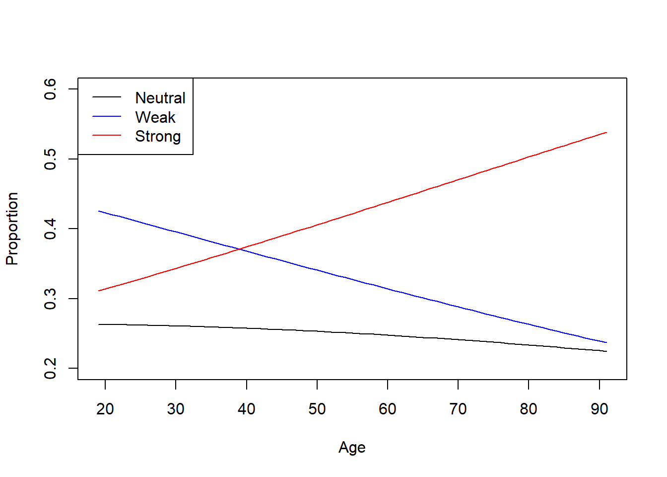
Figure 7.10: Age Group by Predicted Probabilities
Predict for Specific Ages
# Predict class for a 34-year-old
predict(Multinomial_Step, data.frame(age = 34))
#> [1] Weak
#> Levels: Neutral Strong Weak

# Predict probabilities for 34 and 35-year-olds
predict(Multinomial_Step,
        data.frame(age = c(34, 35)),
        type = "probs")
#>     Neutral    Strong      Weak
#> 1 0.2597275 0.3556910 0.3845815
#> 2 0.2594080 0.3587639 0.3818281
7.7.8 Application: Gamma Regression
When response variables are strictly positive, we use Gamma regression.
1. Load and Prepare Data
library(agridat)  # Agricultural dataset
library(ggplot2)

# Load and filter data
dat <- agridat::streibig.competition
gammaDat <- subset(dat, sseeds < 1)  # Keep only barley
gammaDat <-
    transform(gammaDat,
              x = bseeds,
              y = bdwt,
              block = factor(block))
2. Visualization of Inverse Yield
ggplot(gammaDat, aes(x = x, y = 1 / y)) +
    geom_point(aes(color = block, shape = block)) +
    labs(title = "Inverse Yield vs Seeding Rate",
         x = "Seeding Rate",
         y = "Inverse Yield")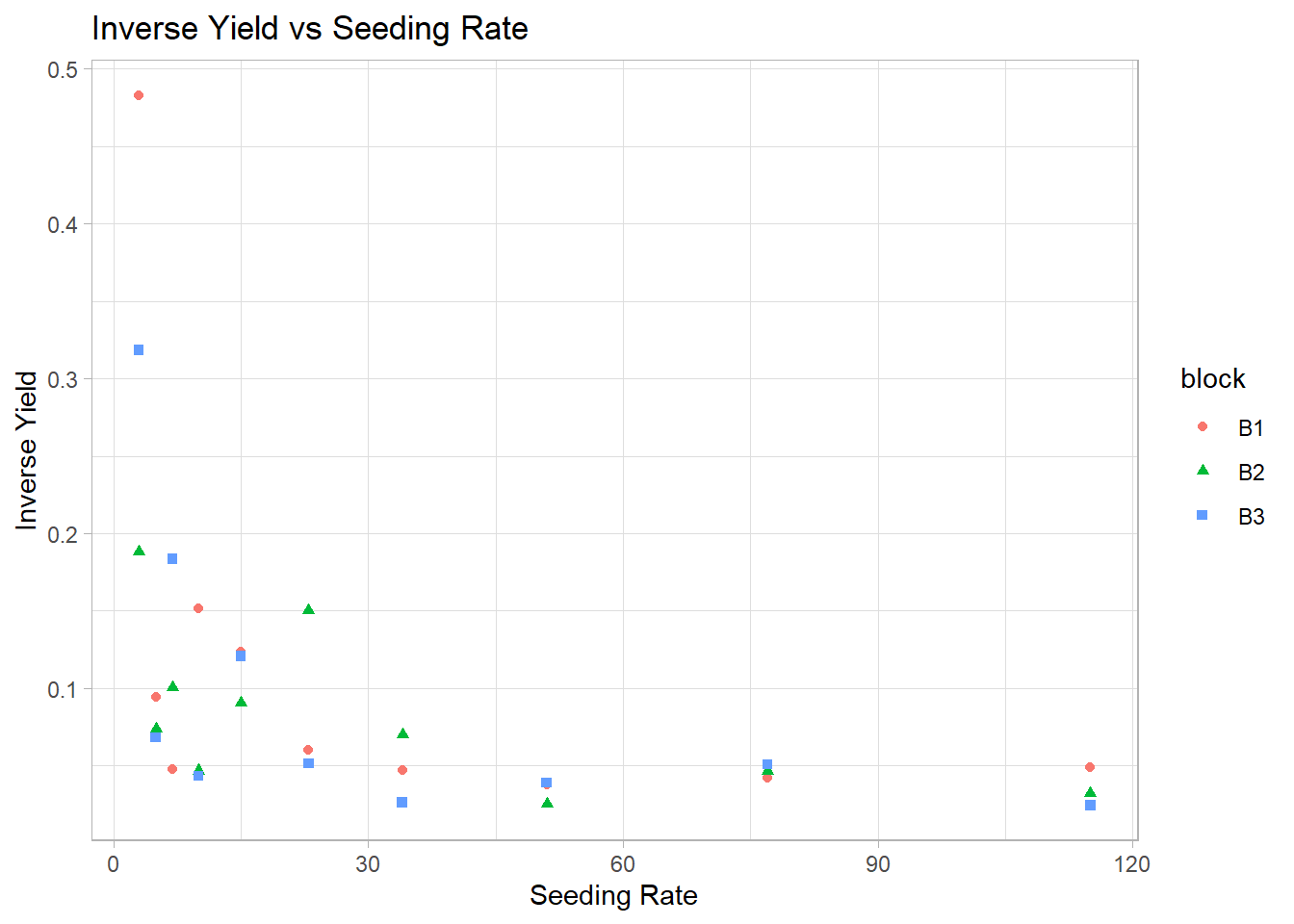
Figure 7.11: Inverse Yield vs Seeding Rate
3. Fit Gamma Regression Model
Gamma regression models yield as a function of seeding rate using an inverse link:
\[ \eta_{ij} = \beta_{0j} + \beta_{1j} x_{ij} + \beta_2 x_{ij}^2, \quad Y_{ij} = \eta_{ij}^{-1} \]
m1 <- glm(y ~ block + block * x + block * I(x^2),
          data = gammaDat, family = Gamma(link = "inverse"))

summary(m1)
#>
#> Call:
#> glm(formula = y ~ block + block * x + block * I(x^2), family = Gamma(link = "inverse"),
#>     data = gammaDat)
#>
#> Coefficients:
#>                  Estimate Std. Error t value Pr(>|t|)
#> (Intercept)     1.115e-01  2.870e-02   3.886 0.000854 ***
#> blockB2        -1.208e-02  3.880e-02  -0.311 0.758630
#> blockB3        -2.386e-02  3.683e-02  -0.648 0.524029
#> x              -2.075e-03  1.099e-03  -1.888 0.072884 .
#> I(x^2)          1.372e-05  9.109e-06   1.506 0.146849
#> blockB2:x       5.198e-04  1.468e-03   0.354 0.726814
#> blockB3:x       7.475e-04  1.393e-03   0.537 0.597103
#> blockB2:I(x^2) -5.076e-06  1.184e-05  -0.429 0.672475
#> blockB3:I(x^2) -6.651e-06  1.123e-05  -0.592 0.560012
#> ---
#> Signif. codes:  0 '***' 0.001 '**' 0.01 '*' 0.05 '.' 0.1 ' ' 1
#>
#> (Dispersion parameter for Gamma family taken to be 0.3232083)
#>
#>     Null deviance: 13.1677  on 29  degrees of freedom
#> Residual deviance:  7.8605  on 21  degrees of freedom
#> AIC: 225.32
#>
#> Number of Fisher Scoring iterations: 5
4. Predictions and Visualization
# Generate new data for prediction
newdf <-
    expand.grid(x = seq(0, 120, length = 50),
                block = factor(c("B1", "B2", "B3")))

# Predict responses
newdf$pred <- predict(m1, newdata = newdf, type = "response")
# Plot predictions
ggplot(gammaDat, aes(x = x, y = y)) +
geom_point(aes(color = block, shape = block)) +
geom_line(data = newdf, aes(
x = x,
y = pred,
color = block,
linetype = block
)) +
labs(title = "Predicted Yield by Seeding Rate",
x = "Seeding Rate",
y = "Yield")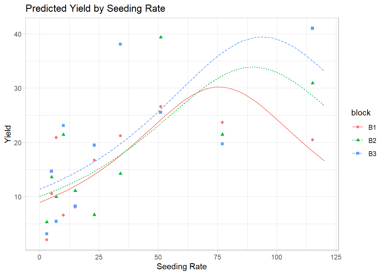
Figure 7.12: Predicted Yield by Seeding Rate