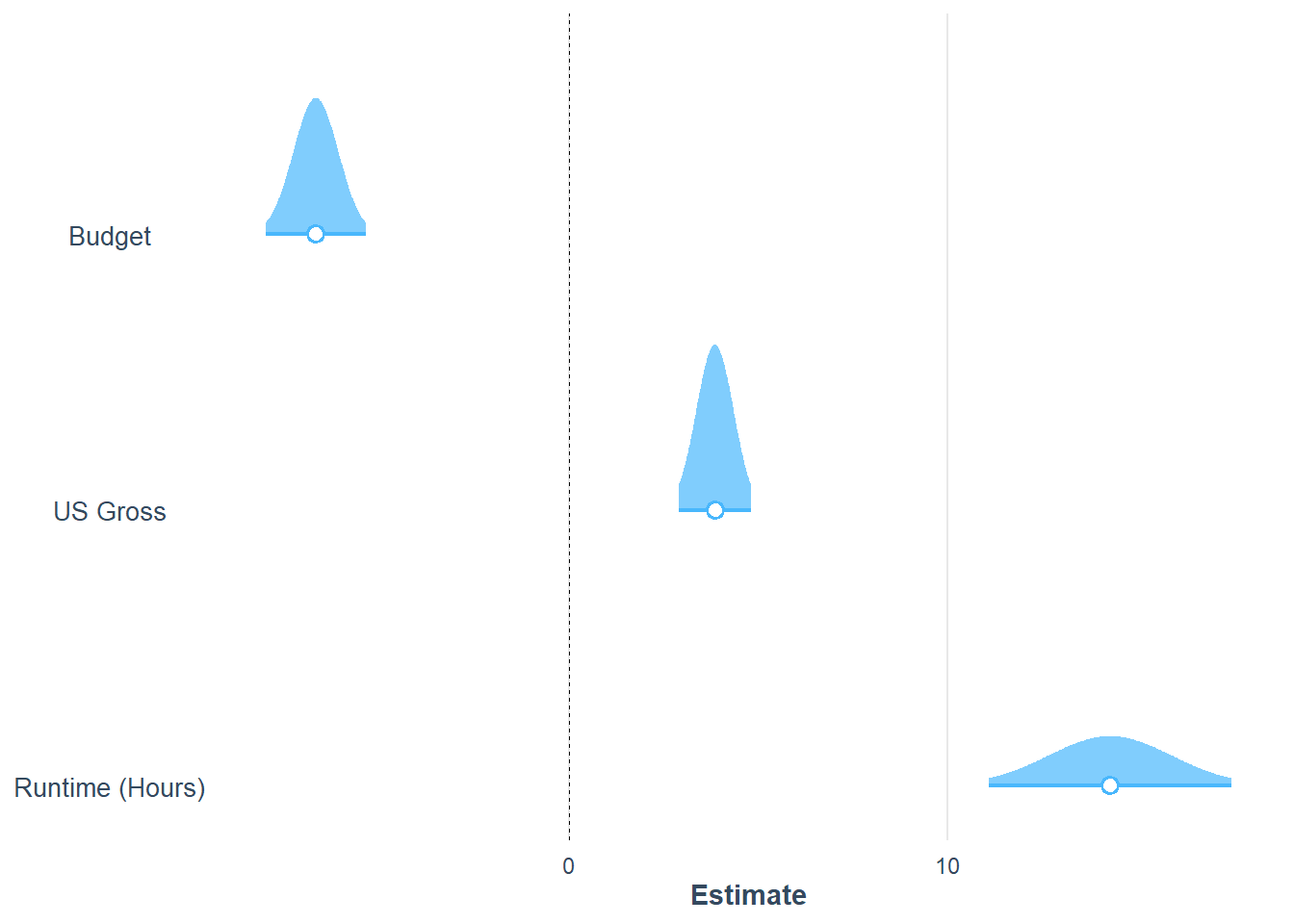
40.6 Changes in an Estimate
Visualize how coefficient estimates shift when adding controls. This is especially useful to show robustness to omitted variable bias concerns.
coef_names_plot <- coef_names[1:3] # Dropping intercept for plots
plot_summs(fit_a, fit_b, fit_c, robust = "HC3", coefs = coef_names_plot)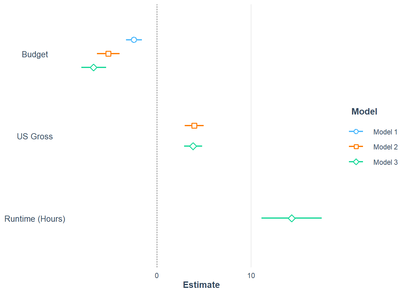
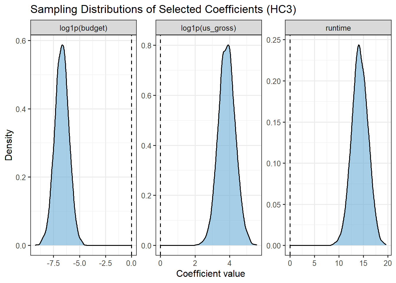
40.6.1 Coefficient Uncertainty and Distribution
Visualize uncertainty with either frequentist or Bayesian approaches. With frequentist OLS, we can simulate coefficient draws from the asymptotic sampling distribution using the estimated variance-covariance matrix and then plot with ggplot2.
# Simulate coefficient draws (multivariate normal approx)
if (requireNamespace("MASS", quietly = TRUE)) {
  V <- vcovHC(fit_c, type = "HC3")
  b <- coef(fit_c)
  draws <- MASS::mvrnorm(n = 5000, mu = b, Sigma = V)
  draws_df <- as.data.frame(draws) %>%
    select(`log1p(budget)`, `log1p(us_gross)`, runtime)

  draws_long <- tidyr::pivot_longer(draws_df, everything(), names_to = "term", values_to = "beta")

  ggplot(draws_long, aes(beta)) +
    facet_wrap(~ term, scales = "free") +
    geom_density(fill = "#6baed6", alpha = 0.6) +
    geom_vline(xintercept = 0, linetype = 2) +
    labs(title = "Sampling Distributions of Selected Coefficients (HC3)",
         x = "Coefficient value", y = "Density") +
    theme_bw(base_size = 12)
}