10.3 Kernel Regression
10.3.1 Basic Setup
A kernel function \(K(\cdot)\) is a non-negative, symmetric function whose integral (or sum, in a discrete setting) equals 1. In nonparametric statistics—such as kernel density estimation or local regression—kernels serve as weighting mechanisms, assigning higher weights to points closer to the target location and lower weights to points farther away. Specifically, a valid kernel function must satisfy:
Non-negativity:
\[ K(u) \ge 0 \quad \text{for all } u. \]Normalization:
\[ \int_{-\infty}^{\infty} K(u)du = 1. \]Symmetry:
\[ K(u) = K(-u) \quad \text{for all } u. \]
In practice, the bandwidth (sometimes called the smoothing parameter) used alongside a kernel usually has a greater impact on the quality of the estimate than the particular form of the kernel. However, choosing a suitable kernel can still influence computational efficiency and the smoothness of the resulting estimates.
10.3.1.1 Common Kernel Functions
A kernel function essentially measures proximity, assigning higher weights to observations \(x_i\) that are close to the target point \(x\), and smaller weights to those farther away.
- Gaussian Kernel \[ K(u) = \frac{1}{\sqrt{2\pi}} e^{-\frac{u^2}{2}}. \]
Shape: Bell-shaped and infinite support (i.e., \(K(u)\) is technically nonzero for all \(u \in (-\infty,\infty)\)), though values decay rapidly as \(|u|\) grows.
Usage: Due to its smoothness and mathematical convenience (especially in closed-form expressions and asymptotic analysis), it is the most widely used kernel in both density estimation and regression smoothing.
Properties: The Gaussian kernel minimizes mean square error in many asymptotic scenarios, making it a common “default choice.”
- Epanechnikov Kernel \[ K(u) = \begin{cases} \frac{3}{4}(1 - u^2) & \text{if } |u| \le 1,\\ 0 & \text{otherwise}. \end{cases} \]
Shape: Parabolic (inverted) on \([-1, 1]\), dropping to 0 at \(|u|=1\).
Usage: Known for being optimal in a minimax sense for certain classes of problems, and it is frequently preferred when compact support (zero weights outside \(|u|\le 1\)) is desirable.
Efficiency: Because it is only supported on a finite interval, computations often involve fewer points (those outside \(|u|\le 1\) have zero weight), which can be computationally more efficient in large datasets.
- Uniform (or Rectangular) Kernel \[ K(u) = \begin{cases} \frac{1}{2} & \text{if } |u| \le 1,\\ 0 & \text{otherwise}. \end{cases} \]
Shape: A simple “flat top” distribution on \([-1, 1]\).
Usage: Sometimes used for its simplicity. In certain methods (e.g., a “moving average” approach), the uniform kernel equates to giving all points within a fixed window the same weight.
Drawback: Lacks smoothness at the boundaries ∣u∣=1|u|=1∣u∣=1, and it can introduce sharper transitions in estimates compared to smoother kernels.
- Triangular Kernel \[ K(u) = \begin{cases} 1 - |u| & \text{if } |u| \le 1,\\ 0 & \text{otherwise}. \end{cases} \]
Shape: Forms a triangle with a peak at \(u=0\) and linearly descends to 0 at \(|u|=1\).
Usage: Provides a continuous but piecewise-linear alternative to the uniform kernel; places relatively more weight near the center compared to the uniform kernel.
- Biweight (or Quartic) Kernel \[ K(u) = \begin{cases} \frac{15}{16} \left(1 - u^2\right)^2 & \text{if } |u| \le 1,\\ 0 & \text{otherwise}. \end{cases} \]
Shape: Smooth and “bump-shaped,” similar to the Epanechnikov but with a steeper drop-off near \(|u|=1\).
Usage: Popular when a smoother, polynomial-based kernel with compact support is desired.
- Cosine Kernel \[ K(u) = \begin{cases} \frac{\pi}{4}\cos\left(\frac{\pi}{2}u\right) & \text{if } |u| \le 1,\\ 0 & \text{otherwise}. \end{cases} \]
Shape: A single “arch” of a cosine wave on the interval \([-1,1]\).
Usage: Used less frequently but can be appealing for certain smoothness criteria or specific signal processing contexts.
Below is a comparison of widely used kernel functions, their functional forms, support, and main characteristics.
| Kernel | Formula | Support | Key Characteristics |
|---|---|---|---|
| Gaussian | \(\displaystyle K(u) = \frac{1}{\sqrt{2\pi}} e^{-\frac{u^2}{2}}\) | \(u \in (-\infty,\infty)\) | Smooth, bell-shaped | | | | | Nonzero for all \(u\), but decays quickly | | | | Often the default choice due to favorable analytical properties | ||
| Epanechnikov | \(\displaystyle K(u) = \begin{cases}\frac{3}{4}(1 - u^2) & |u|\le 1 \\ 0 & \text{otherwise}\end{cases}\) | \([-1,1]\) | Parabolic shape Compact support Minimizes mean integrated squared error in certain theoretical contexts |
| Uniform | \(\displaystyle K(u) = \begin{cases}\tfrac{1}{2} & |u|\le 1 \\ 0 & \text{otherwise}\end{cases}\) | \([-1,1]\) | Flat (rectangular) shape Equal weight for all points within \([-1,1]\) Sharp boundary can lead to less smooth estimates |
| Triangular | \(\displaystyle K(u) = \begin{cases}1 - |u| & |u|\le 1 \\ 0 & \text{otherwise}\end{cases}\) | \([-1,1]\) | Linear decrease from the center \(u=0\) to 0 at \(|u|=1\) Compact support A bit smoother than the uniform kernel |
| Biweight (Quartic) | \(\displaystyle K(u) = \begin{cases}\frac{15}{16}(1 - u^2)^2 & |u|\le 1 \\ 0 & \text{otherwise}\end{cases}\) | \([-1,1]\) | Polynomial shape, smooth Compact support Often used for its relatively smooth taper near the boundaries |
| Cosine | \(\displaystyle K(u) = \begin{cases}\frac{\pi}{4}\cos\left(\frac{\pi}{2}u\right) & |u|\le 1 \\ 0 & \text{otherwise}\end{cases}\) | \([-1,1]\) | Single arch of a cosine wave Compact support Less commonly used, but still mathematically straightforward |
10.3.1.2 Additional Details and Usage Notes
- Smoothness and Differentiability
- Kernels with infinite support (like the Gaussian) can yield very smooth estimates but require summing over (practically) all data points.
- Kernels with compact support (like Epanechnikov, biweight, triangular, etc.) go to zero outside a fixed interval. This can make computations more efficient since only data within a certain range of the target point matter.
- Choice of Kernel vs. Choice of Bandwidth
- While the kernel shape does have some effect on the estimator’s smoothness, the choice of bandwidth (sometimes denoted \(h\)) is typically more critical. If \(h\) is too large, the estimate can be excessively smooth (high bias). If \(h\) is too small, the estimate can exhibit high variance or appear “noisy.”
- Local Weighting Principle
- At a target location \(x\), a kernel function \(K\left(\frac{x - x_i}{h}\right)\) down-weights data points \((x_i)\) that are farther from \(x\). Nearer points have larger kernel values, hence exert greater influence on the local estimate.
- Interpretation in Density Estimation
- In kernel density estimation, each data point contributes a small “bump” (shaped by the kernel) to the overall density. Summing or integrating these bumps yields a continuous estimate of the underlying density function, in contrast to discrete histograms.
10.3.2 Nadaraya-Watson Kernel Estimator
The most widely used kernel-based regression estimator is the Nadaraya-Watson estimator (Nadaraya 1964; Watson 1964), defined as:
\[ \hat{m}_h(x) = \frac{\sum_{i=1}^n K\!\left(\frac{x - x_i}{h}\right) y_i}{\sum_{i=1}^n K\!\left(\frac{x - x_i}{h}\right)}, \]
where \(h > 0\) is the bandwidth parameter. Intuitively, this formula computes a weighted average of the observed \(y_i\) values, with weights determined by the kernel function applied to the scaled distance between \(x\) and each \(x_i\).
Interpretation:
- When \(|x - x_i|\) is small (i.e., \(x_i\) is close to \(x\)), the kernel value \(K\!\left(\frac{x - x_i}{h}\right)\) is large, giving more weight to \(y_i\).
- When \(|x - x_i|\) is large, the kernel value becomes small (or even zero for compactly supported kernels like the Epanechnikov), reducing the influence of \(y_i\) on \(\hat{m}_h(x)\).
Thus, observations near \(x\) have a larger impact on the estimated value \(\hat{m}_h(x)\) than distant ones.
10.3.2.1 Weights Representation
We can define the normalized weights:
\[ w_i(x) = \frac{K\!\left(\frac{x - x_i}{h}\right)}{\sum_{j=1}^n K\!\left(\frac{x - x_j}{h}\right)}, \]
so that the estimator can be rewritten as:
\[ \hat{m}_h(x) = \sum_{i=1}^n w_i(x) y_i, \]
where \(\sum_{i=1}^n w_i(x) = 1\) for any \(x\). Notice that \(0 \le w_i(x) \le 1\) for all \(i\).
10.3.3 Priestley–Chao Kernel Estimator
The Priestley–Chao kernel estimator (Priestley and Chao 1972) is an early kernel-based regression estimator designed to estimate the regression function \(m(x)\) from observed data \(\{(x_i, y_i)\}_{i=1}^n\). Unlike the Nadaraya–Watson estimator, which uses pointwise kernel weighting, the Priestley–Chao estimator incorporates differences in the predictor variable to approximate integrals more accurately.
The estimator is defined as:
\[ \hat{m}_h(x) = \frac{1}{h} \sum_{i=1}^{n-1} K\!\left(\frac{x - x_i}{h}\right) \cdot (x_{i+1} - x_i) \cdot y_i, \]
where:
\(K(\cdot)\) is a kernel function,
\(h > 0\) is the bandwidth parameter,
\((x_{i+1} - x_i)\) represents the spacing between consecutive observations.
10.3.3.1 Interpretation
- The estimator can be viewed as a Riemann sum approximation of an integral, where the kernel-weighted \(y_i\) values are scaled by the spacing \((x_{i+1} - x_i)\).
- Observations where \(x_i\) is close to \(x\) receive more weight due to the kernel function.
- The inclusion of \((x_{i+1} - x_i)\) accounts for non-uniform spacing in the data, making the estimator more accurate when the predictor values are irregularly spaced.
This estimator is particularly useful when the design points \(\{x_i\}\) are unevenly distributed.
10.3.3.2 Weights Representation
We can express the estimator as a weighted sum of the observed responses \(y_i\):
\[ \hat{m}_h(x) = \sum_{i=1}^{n-1} w_i(x) y_i, \]
where the weights are defined as:
\[ w_i(x) = \frac{1}{h} \cdot K\!\left(\frac{x - x_i}{h}\right) \cdot (x_{i+1} - x_i). \]
Properties of the weights:
Non-negativity: If \(K(u) \ge 0\), then \(w_i(x) \ge 0\).
Adaptation to spacing: Larger gaps \((x_{i+1} - x_i)\) increase the corresponding weight.
Unlike Nadaraya–Watson, the weights do not sum to 1, as they approximate an integral rather than a normalized average.
10.3.4 Gasser–Müller Kernel Estimator
The Gasser–Müller kernel estimator (Gasser and Müller 1979) improves upon the Priestley–Chao estimator by using a cumulative kernel function to smooth over the predictor space. This estimator is particularly effective for irregularly spaced data and aims to reduce bias at the boundaries.
The estimator is defined as:
\[ \hat{m}_h(x) = \frac{1}{h} \sum_{i=1}^{n-1} \left[ K^*\!\left(\frac{x - x_i}{h}\right) - K^*\!\left(\frac{x - x_{i+1}}{h}\right) \right] \cdot y_i, \]
where:
\(K^*(u) = \int_{-\infty}^{u} K(v) dv\) is the cumulative distribution function (CDF) of the kernel \(K\),
\(h > 0\) is the bandwidth parameter.
10.3.4.1 Interpretation
- The estimator computes the difference of cumulative kernel functions at two consecutive design points, effectively assigning weight to the interval between \(x_i\) and \(x_{i+1}\).
- Observations contribute more to \(\hat{m}_h(x)\) when \(x\) lies between \(x_i\) and \(x_{i+1}\), with the contribution decreasing as the distance from \(x\) increases.
- This method smooths over intervals rather than just at points, reducing bias near the boundaries and improving performance with unevenly spaced data.
10.3.4.2 Weights Representation
The Gasser–Müller estimator can also be expressed as a weighted sum:
\[ \hat{m}_h(x) = \sum_{i=1}^{n-1} w_i(x) y_i, \]
where the weights are:
\[ w_i(x) = \frac{1}{h} \left[ K^*\!\left(\frac{x - x_i}{h}\right) - K^*\!\left(\frac{x - x_{i+1}}{h}\right) \right]. \]
Properties of the weights:
Non-negativity: The weights are non-negative if \(K^*\) is non-decreasing (which holds if \(K\) is non-negative).
Adaptation to spacing: The weights account for the spacing between \(x_i\) and \(x_{i+1}\).
Similar to the Priestley–Chao estimator, the weights do not sum to 1 because the estimator approximates an integral rather than a normalized sum.
10.3.5 Comparison of Kernel-Based Estimators
| Estimator | Formula | Key Feature | Weights Sum to 1? |
|---|---|---|---|
| Nadaraya–Watson | \(\displaystyle \hat{m}_h(x) = \frac{\sum K\left(\frac{x - x_i}{h}\right) y_i}{\sum K\left(\frac{x - x_i}{h}\right)}\) | Weighted average of \(y_i\) | Yes |
| Priestley–Chao | \(\displaystyle \hat{m}_h(x) = \frac{1}{h} \sum K\left(\frac{x - x_i}{h}\right)(x_{i+1} - x_i) y_i\) | Incorporates data spacing | No |
| Gasser–Müller | \(\displaystyle \hat{m}_h(x) = \frac{1}{h} \sum \left[K^*\left(\frac{x - x_i}{h}\right) - K^*\left(\frac{x - x_{i+1}}{h}\right)\right] y_i\) | Uses cumulative kernel differences | No |
10.3.6 Bandwidth Selection
The choice of bandwidth \(h\) is crucial because it controls the trade-off between bias and variance:
- If \(h\) is too large, the estimator becomes overly smooth, incorporating too many distant data points. This leads to high bias but low variance.
- If \(h\) is too small, the estimator becomes noisy and sensitive to fluctuations in the data, resulting in low bias but high variance.
10.3.6.1 Mean Squared Error and Optimal Bandwidth
To analyze the performance of kernel estimators, we often examine the mean integrated squared error (MISE):
\[ \text{MISE}(\hat{m}_h) = \mathbb{E}\left[\int \left\{\hat{m}_h(x) - m(x)\right\}^2 dx \right]. \]
As \(n \to \infty\), under smoothness assumptions on \(m(x)\) and regularity conditions on the kernel \(K\), the MISE has the following asymptotic expansion:
\[ \text{MISE}(\hat{m}_h) \approx \frac{R(K)}{n h} \sigma^2 + \frac{1}{4} \mu_2^2(K) h^4 \int \left\{m''(x)\right\}^2 dx, \]
where:
- \(R(K) = \int_{-\infty}^{\infty} K(u)^2 du\) measures the roughness of the kernel.
- \(\mu_2(K) = \int_{-\infty}^{\infty} u^2 K(u) du\) is the second moment of the kernel (related to its spread).
- \(\sigma^2\) is the variance of the noise, assuming \(\operatorname{Var}(\varepsilon \mid X = x) = \sigma^2\).
- \(m''(x)\) is the second derivative of the true regression function \(m(x)\).
To find the asymptotically optimal bandwidth, we differentiate the MISE with respect to \(h\), set the derivative to zero, and solve for \(h\):
\[ h_{\mathrm{opt}} = \left(\frac{R(K) \sigma^2}{\mu_2^2(K) \int \left\{m''(x)\right\}^2 dx} \cdot \frac{1}{n}\right)^{1/5}. \]
In practice, \(\sigma^2\) and \(\int \{m''(x)\}^2 dx\) are unknown and must be estimated from data. A common data-driven approach is cross-validation.
10.3.6.2 Cross-Validation
The leave-one-out cross-validation (LOOCV) method is widely used for bandwidth selection:
- For each \(i = 1, \dots, n\), fit the kernel estimator \(\hat{m}_{h,-i}(x)\) using all data except the \(i\)-th observation \((x_i, y_i)\).
- Compute the squared prediction error for the left-out point: \((y_i - \hat{m}_{h,-i}(x_i))^2\).
- Average these errors across all observations:
\[ \mathrm{CV}(h) = \frac{1}{n} \sum_{i=1}^n \left\{y_i - \hat{m}_{h,-i}(x_i)\right\}^2. \]
The bandwidth \(h\) that minimizes \(\mathrm{CV}(h)\) is selected as the optimal bandwidth.
10.3.7 Asymptotic Properties
For the Nadaraya-Watson estimator, under regularity conditions and assuming \(h \to 0\) as \(n \to \infty\) (but not too fast), we have:
Consistency: \[ \hat{m}_h(x) \overset{p}{\longrightarrow} m(x), \] meaning the estimator converges in probability to the true regression function.
Rate of Convergence: The mean squared error (MSE) decreases at the rate: \[ \text{MSE}(\hat{m}_h(x)) = O\left(n^{-4/5}\right) \] in the one-dimensional case. This rate results from balancing the variance term (\(O(1/(nh))\)) and the squared bias term (\(O(h^4)\)).
10.3.8 Derivation of the Nadaraya-Watson Estimator
The Nadaraya-Watson estimator can be derived from a density-based perspective:
By the definition of conditional expectation: \[ m(x) = \mathbb{E}[Y \mid X = x] = \frac{\int y f_{X,Y}(x, y) dy}{f_X(x)}, \] where \(f_{X,Y}(x, y)\) is the joint density of \((X, Y)\), and \(f_X(x)\) is the marginal density of \(X\).
Estimate \(f_X(x)\) using a kernel density estimator: \[ \hat{f}_X(x) = \frac{1}{n} \sum_{i=1}^n \frac{1}{h} K\!\left(\frac{x - x_i}{h}\right). \]
Estimate the joint density \(f_{X,Y}(x, y)\): \[ \hat{f}_{X,Y}(x, y) = \frac{1}{n} \sum_{i=1}^n \frac{1}{h} K\!\left(\frac{x - x_i}{h}\right) \delta_{y_i}(y), \] where \(\delta_{y_i}(y)\) is the Dirac delta function (a point mass at \(y_i\)).
The kernel regression estimator becomes: \[ \hat{m}_h(x) = \frac{\int y \hat{f}_{X,Y}(x, y) dy}{\hat{f}_X(x)} = \frac{\sum_{i=1}^n K\!\left(\frac{x - x_i}{h}\right) y_i}{\sum_{i=1}^n K\!\left(\frac{x - x_i}{h}\right)}, \] which is exactly the Nadaraya-Watson estimator.
# Load necessary libraries
library(ggplot2)
library(gridExtra)


# 1. Simulate Data
set.seed(123)


# Generate predictor x and response y
n <- 100
x <-
    sort(runif(n, 0, 10))  # Sorted for Priestley–Chao and Gasser–Müller
true_function <-
    function(x)
        sin(x) + 0.5 * cos(2 * x)  # True regression function

# Add Gaussian noise
y <-
    true_function(x) + rnorm(n, sd = 0.3)
# Visualization of the data
ggplot(data.frame(x, y), aes(x, y)) +
geom_point(color = "darkblue") +
geom_line(aes(y = true_function(x)),
color = "red",
linetype = "dashed") +
labs(title = "Simulated Data with True Regression Function",
x = "x", y = "y") +
theme_minimal()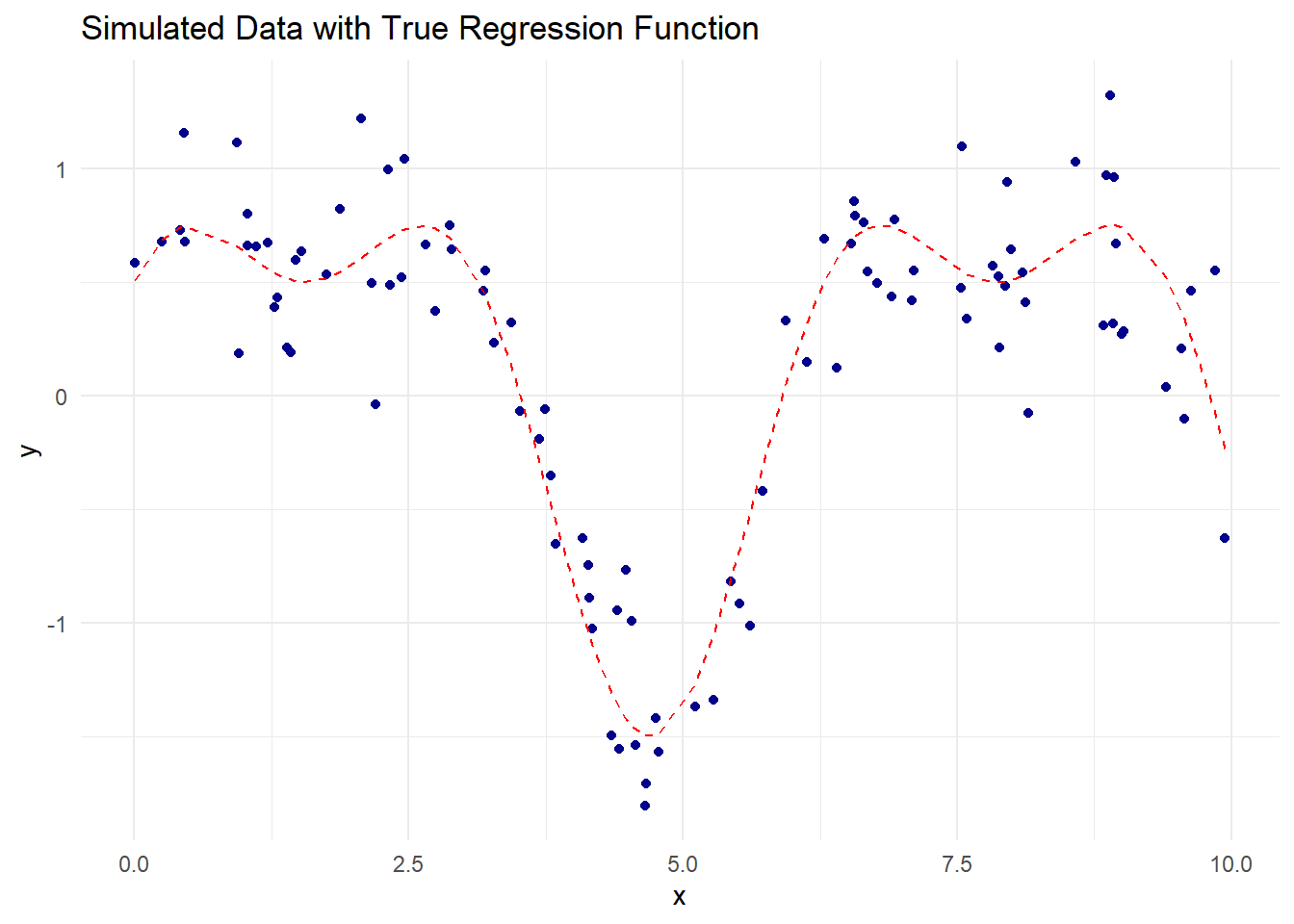
Figure 10.1: Simulated Data with True Regression Function
# Gaussian Kernel Function
gaussian_kernel <- function(u) {
    (1 / sqrt(2 * pi)) * exp(-0.5 * u ^ 2)
}

# Epanechnikov Kernel Function
epanechnikov_kernel <- function(u) {
    ifelse(abs(u) <= 1, 0.75 * (1 - u ^ 2), 0)
}

# Cumulative Kernel for Gasser–Müller (CDF of Gaussian Kernel)
gaussian_cdf_kernel <- function(u) {
    pnorm(u, mean = 0, sd = 1)
}
# Nadaraya-Watson Estimator
nadaraya_watson <-
function(x_eval, x, y, h, kernel = gaussian_kernel) {
sapply(x_eval, function(x0) {
weights <- kernel((x0 - x) / h)
sum(weights * y) / sum(weights)
})
}
# Bandwidth Selection (fixed for simplicity)
h_nw <- 0.5 # Bandwidth for Nadaraya–Watson
# Apply Nadaraya–Watson Estimator
x_grid <- seq(0, 10, length.out = 200)
nw_estimate <- nadaraya_watson(x_grid, x, y, h_nw)# Plot Nadaraya–Watson Estimate
ggplot() +
geom_point(aes(x, y), color = "darkblue", alpha = 0.6) +
geom_line(aes(x_grid, nw_estimate),
color = "green",
linewidth = 1.2) +
geom_line(aes(x_grid, true_function(x_grid)),
color = "red",
linetype = "dashed") +
labs(
title = "Nadaraya–Watson Kernel Estimator",
subtitle = paste("Bandwidth (h) =", h_nw),
x = "x",
y = "Estimated m(x)"
) +
theme_minimal()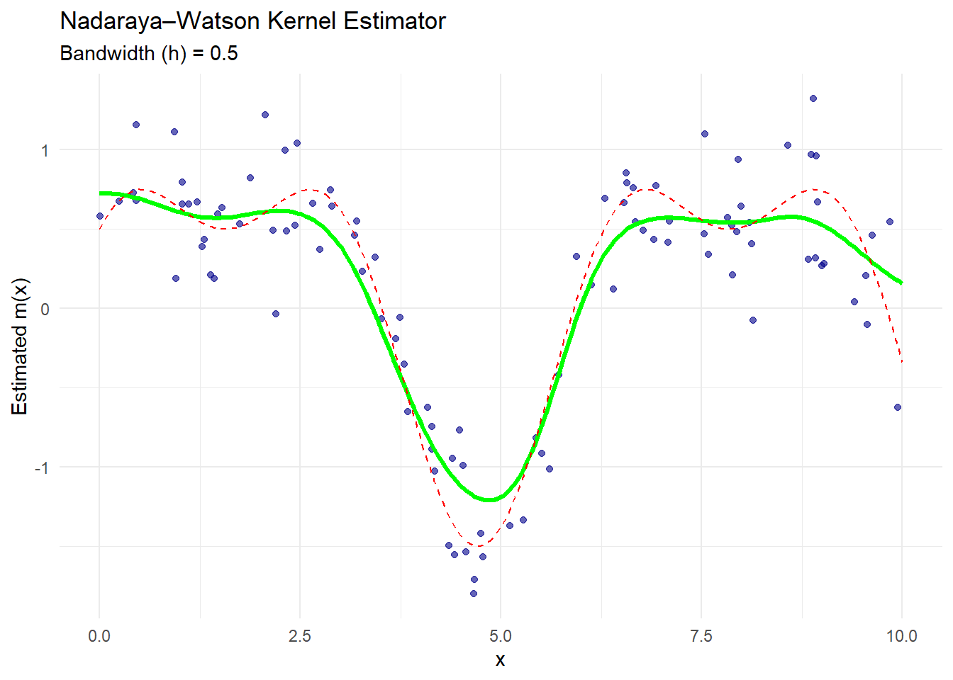
Figure 10.2: Nadaraya–Watson Kernel Estimator
The green curve is the Nadaraya–Watson estimate.
The dashed red line is the true regression function.
The blue dots are the observed noisy data.
The estimator smooths the data, assigning more weight to points close to each evaluation point based on the Gaussian kernel.
# Priestley–Chao Estimator
priestley_chao <-
    function(x_eval, x, y, h, kernel = gaussian_kernel) {
        sapply(x_eval, function(x0) {
            weights <- kernel((x0 - x[-length(x)]) / h) * diff(x)
            sum(weights * y[-length(y)]) / h
        })
    }

# Apply Priestley–Chao Estimator
h_pc <- 0.5
pc_estimate <- priestley_chao(x_grid, x, y, h_pc)
# Plot Priestley–Chao Estimate
ggplot() +
geom_point(aes(x, y), color = "darkblue", alpha = 0.6) +
geom_line(aes(x_grid, pc_estimate),
color = "orange",
linewidth = 1.2) +
geom_line(aes(x_grid, true_function(x_grid)),
color = "red",
linetype = "dashed") +
labs(
title = "Priestley–Chao Kernel Estimator",
subtitle = paste("Bandwidth (h) =", h_pc),
x = "x",
y = "Estimated m(x)"
) +
theme_minimal()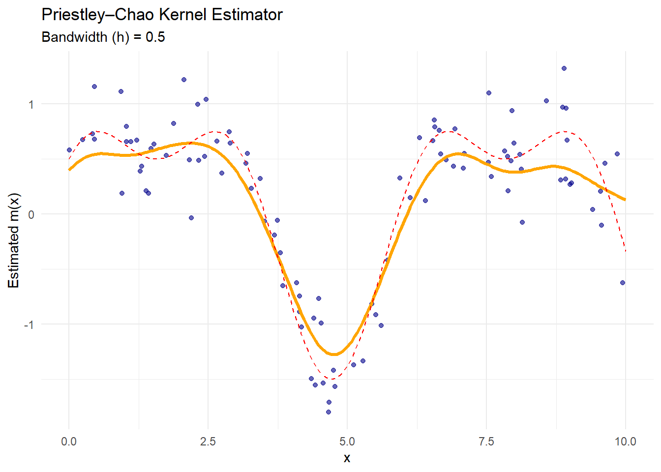
Figure 10.3: Priestley–Chao Kernel Estimator
The orange curve is the Priestley–Chao estimate.
This estimator incorporates the spacing between consecutive data points (
diff(x)), making it more sensitive to non-uniform data spacing.It performs similarly to Nadaraya–Watson when data are evenly spaced.
# Gasser–Müller Estimator
gasser_mueller <-
    function(x_eval, x, y, h, cdf_kernel = gaussian_cdf_kernel) {
        sapply(x_eval, function(x0) {
            weights <-
                (cdf_kernel((x0 - x[-length(x)]) / h) - cdf_kernel((x0 - x[-1]) / h))
            sum(weights * y[-length(y)]) / h
        })
    }

# Apply Gasser–Müller Estimator
h_gm <- 0.5
gm_estimate <- gasser_mueller(x_grid, x, y, h_gm)
# Plot Gasser–Müller Estimate
ggplot() +
geom_point(aes(x, y), color = "darkblue", alpha = 0.6) +
geom_line(aes(x_grid, gm_estimate),
color = "purple",
size = 1.2) +
geom_line(aes(x_grid, true_function(x_grid)),
color = "red",
linetype = "dashed") +
labs(
title = "Gasser–Müller Kernel Estimator",
subtitle = paste("Bandwidth (h) =", h_gm),
x = "x",
y = "Estimated m(x)"
) +
theme_minimal()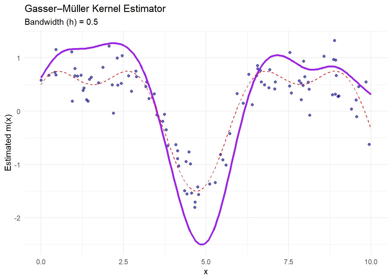
Figure 10.4: Gasser–Müller Kernel Estimator
The purple curve is the Gasser–Müller estimate.
This estimator uses cumulative kernel functions to handle irregular data spacing and reduce boundary bias.
It performs well when data are unevenly distributed.
# Combine all estimates for comparison
estimates_df <- data.frame(
    x = x_grid,
    Nadaraya_Watson = nw_estimate,
    Priestley_Chao = pc_estimate,
    Gasser_Mueller = gm_estimate,
    True_Function = true_function(x_grid)
)
# Plot all estimators together
ggplot() +
geom_point(aes(x, y), color = "gray60", alpha = 0.5) +
geom_line(aes(x, Nadaraya_Watson, color = "Nadaraya–Watson"),
data = estimates_df, size = 1.1) +
geom_line(aes(x, Priestley_Chao, color = "Priestley–Chao"),
data = estimates_df, size = 1.1) +
geom_line(aes(x, Gasser_Mueller, color = "Gasser–Müller"),
data = estimates_df, size = 1.1) +
geom_line(aes(x, True_Function, color = "True Function"),
data = estimates_df, linetype = "dashed", size = 1) +
scale_color_manual(
name = "Estimator",
values = c("Nadaraya–Watson" = "green",
"Priestley–Chao" = "orange",
"Gasser–Müller" = "purple",
"True Function" = "red")
) +
labs(
title = "Comparison of Kernel-Based Regression Estimators",
x = "x",
y = "Estimated m(x)"
) +
theme_minimal()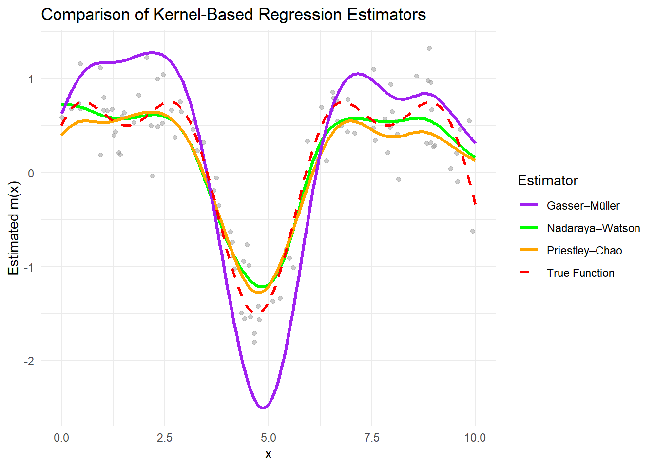
Figure 10.5: Comparison of Kernel-Based Regression Estimators
All estimators approximate the true function well when the bandwidth is appropriately chosen.
The Nadaraya–Watson estimator is sensitive to bandwidth selection and assumes uniform data spacing.
The Priestley–Chao estimator accounts for data spacing, making it more flexible with uneven data.
The Gasser–Müller estimator reduces boundary bias and handles irregular data effectively.
# Cross-validation for bandwidth selection (for Nadaraya–Watson)
cv_bandwidth <- function(h, x, y, kernel = gaussian_kernel) {
  n <- length(y)
  cv_error <- 0
  for (i in 1:n) {
    x_train <- x[-i]
    y_train <- y[-i]
    y_pred <- nadaraya_watson(x[i], x_train, y_train, h, kernel)
    cv_error <- cv_error + (y[i] - y_pred)^2
  }
  return(cv_error / n)
}

# Optimize bandwidth
bandwidths <- seq(0.1, 2, by = 0.1)
cv_errors <- sapply(bandwidths, cv_bandwidth, x = x, y = y)

# Optimal bandwidth
optimal_h <- bandwidths[which.min(cv_errors)]
optimal_h
#> [1] 0.3
# Plot CV errors
ggplot(data.frame(bandwidths, cv_errors), aes(bandwidths, cv_errors)) +
geom_line(color = "blue") +
geom_point(aes(x = optimal_h, y = min(cv_errors)),
color = "red",
size = 3) +
labs(title = "Cross-Validation for Bandwidth Selection",
x = "Bandwidth (h)", y = "CV Error") +
theme_minimal()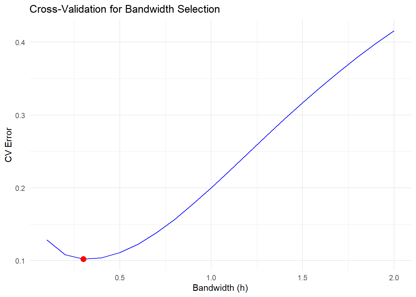
Figure 10.6: Cross-Validation for Bandwidth Selection
The red point indicates the optimal bandwidth that minimizes the cross-validation error.
Selecting the right bandwidth is critical, as it balances bias and variance in the estimator.