16.1 Null Hypothesis Significance Testing
Null Hypothesis Significance Testing (NHST) is the foundation of statistical inference. It provides a structured approach to evaluating whether observed data provides sufficient evidence to reject a null hypothesis (\(H_0\)) in favor of an alternative hypothesis (\(H_a\)).
NHST follows these key steps:
- Define Hypotheses
- The null hypothesis (\(H_0\)) represents the default assumption (e.g., no effect, no difference).
- The alternative hypothesis (\(H_a\)) represents the competing claim (e.g., a nonzero effect, a relationship between variables).
- Select a Test Statistic
- The test statistic (e.g., \(T\), \(W\), \(F\)) quantifies evidence against \(H_0\).
- It follows a known distribution under \(H_0\) (e.g., normal, chi-square, F-distribution).
- Decision Rule & p-value
- If the test statistic exceeds a critical value or the p-value is below \(\alpha\), we reject \(H_0\).
- Otherwise, we fail to reject \(H_0\), meaning the evidence is insufficient to rule it out.
16.1.1 Error Types in Hypothesis Testing
In hypothesis testing, we may incorrectly reject or fail to reject the null hypothesis, leading to two types of errors:
- Type I Error (False Positive):
- Rejecting \(H_0\) when it is actually true.
- Example: Concluding an effect exists when it does not.
- Type II Error (False Negative):
- Failing to reject \(H_0\) when it is actually false.
- Example: Missing a real effect because the test lacked power.
The power of a test is the probability of correctly rejecting \(H_0\) when it is false:
\[ \text{Power} = 1 - P(\text{Type II Error}) \]
A higher power (typically \(\geq 0.8\)) reduces Type II errors and increases the likelihood of detecting true effects.
16.1.2 Hypothesis Testing Framework
Hypothesis tests can be two-sided or one-sided, depending on the research question.
16.1.2.1 Two-Sided Test
In a two-sided test, we examine whether a parameter is significantly different from a hypothesized value (usually zero):
\[ \begin{aligned} &H_0: \beta_j = 0 \\ &H_1: \beta_j \neq 0 \end{aligned} \]
Under the null hypothesis, and assuming standard ordinary least squares assumptions (A1-A3a, A5), the asymptotic distribution of the OLS estimator is:
\[ \sqrt{n} \hat{\beta_j} \sim N(0, \text{Avar}(\sqrt{n} \hat{\beta}_j)) \]
where \(\text{Avar}(\cdot)\) denotes the asymptotic variance.
16.1.2.2 One-Sided Test
For a one-sided hypothesis test, the null hypothesis includes a range of values, and we test against a directional alternative:
\[ \begin{aligned} &H_0: \beta_j \geq 0 \\ &H_1: \beta_j < 0 \end{aligned} \]
The “hardest” null value to reject is \(\beta_j = 0\). Under this specific null, the estimator follows the same asymptotic distribution:
\[ \sqrt{n} \hat{\beta_j} \sim N(0, \text{Avar}(\sqrt{n} \hat{\beta}_j)) \]
16.1.3 Interpreting Hypothesis Testing Results
When conducting hypothesis tests, it is essential to distinguish between population parameters and sample estimates:
- Hypotheses are always written in terms of the population parameter (\(\beta\)), not the sample estimate (\(\hat{\beta}\)).
- Some disciplines use different notations:
- \(\beta\): Standardized coefficient (useful for comparing relative effects, scale-free).
- \(\mathbf{b}\): Unstandardized coefficient (more interpretable in practical applications, e.g., policy decisions).
The relationship between these coefficients is:
\[ \beta_j = \mathbf{b}_j \frac{s_{x_j}}{s_y} \]
where \(s_{x_j}\) and \(s_y\) are the standard deviations of the independent and dependent variables.
16.1.4 Understanding p-Values
The p-value is the probability, under the assumption that \(H_0\) is true, of observing a test statistic at least as extreme as the one computed from the sample data. Formally,
\[ p\text{-value} = P(\text{Test Statistic} \geq \text{observed value} \mid H_0 \ \text{is true}) \]
Interpretation
A small p-value indicates that if \(H_0\) were true, seeing the observed data (or something more extreme) would be unlikely.
By convention, if \(p < \alpha\) (often 0.05), the result is deemed “statistically significant,” and we reject \(H_0\).
Important Caveat: “Statistically significant” is not the same as “practically significant” or “economically significant.” A difference can be statistically significant yet trivial in magnitude, with negligible real-world implications.
Misconceptions
The p-value is not the probability that \(H_0\) is true or false.
A p-value above \(0.05\) does not prove that there is “no effect.” It simply suggests that the data do not provide sufficient evidence (at the chosen significance level) to reject \(H_0\).
A p-value below 0.05 does not prove that an effect is “real” or large. It indicates that the data are unusual enough under \(H_0\) that we decide to reject \(H_0\), given our chosen threshold.
16.1.5 The Role of Sample Size
A critical factor influencing the outcome of hypothesis tests is sample size (\(n\)).
Increasing Power with Large \(n\)
Statistical Power: The probability of correctly rejecting \(H_0\) when \(H_0\) is false. Large sample sizes increase statistical power, making it easier to detect even tiny deviations from \(H_0\).
Implication: If the true effect size in the population is very small (e.g., a 0.2% difference in average returns between two trading strategies), a study with a large enough \(n\) might still find it statistically significant (p-value < 0.05).
Tendency Toward Over-Sensitivity
As \(n\) grows, the standard errors decrease. Thus, even minuscule differences from the null hypothesis become less likely to be attributed to random chance, yielding low p-values. This can lead to findings that are statistically significant but have negligible real-world impact.
- Example: Suppose an economist is testing if a policy intervention changes employment rates by 0.1%. With a small sample size, the test might not detect this difference. But with a massive dataset, the same 0.1% difference might yield a \(p\)-value < 0.05, even though a 0.1% change may not be economically meaningful.
16.1.6 p-Value Hacking
p-Hacking refers to the process of manipulating data analysis until a statistically significant result (\(p\)-value < 0.05) is achieved. This can include:
Running multiple tests on the same dataset and only reporting those that yield significance.
Stopping data collection once a significant p-value is reached.
Trying various model specifications (e.g., adding or removing control variables) until one finds a significant effect.
Selectively reporting outcomes (publication bias).
With large datasets, the “search space” for potential analyses grows exponentially. If researchers test many hypotheses or sift through a wide range of variables and subgroups, they can almost always find a “significant” result by chance alone.
- Multiple Comparison Problem: When multiple tests are conducted, the chance of finding at least one “significant” result purely by coincidence increases. For instance, with 20 independent tests at \(\alpha = .05\), there is a 64% chance (\(1 - 0.95^{20}\)) of incorrectly rejecting at least one null hypothesis.
16.1.7 Practical vs. Statistical Significance
In economics and finance, it is crucial to distinguish between results that are statistically significant and those that are economically meaningful. Economic or financial significance asks: Does this effect have tangible importance to policymakers, businesses, or investors?
- A result might show that a new trading algorithm yields returns that are statistically different from zero, but if that difference is 0.0001% on average, it might not be profitable after accounting for transaction fees, taxes, or other frictions—hence lacking economic significance.
16.1.8 Mitigating the Misuse of p-Values
16.1.8.1 Pre-Registration and Replication
Pre-Registration: Researchers specify hypotheses and analytical methods before seeing the data, reducing the temptation to p-hack.
Replication: Independent replication studies help confirm whether a result is robust or merely a fluke.
16.1.8.2 Using Alternatives to (or Supplements for) p-Values
Bayesian Methods: Provide posterior probabilities that incorporate prior information, often giving a more nuanced understanding of uncertainty.
Effect Size & Confidence Intervals: Shift the focus from “Is it significant?” to “How large is the effect, and what is its plausible range?”
Equivalence Testing: Sometimes the goal is to show the effect is not larger than a certain threshold. Equivalence tests can be used to conclude “no clinically (or economically) significant difference.”
16.1.8.3 Adjusting for Multiple Comparisons
Bonferroni Correction: Requires using a more stringent significance threshold when multiple tests are performed (e.g., \(\alpha/m\) for \(m\) tests).
False Discovery Rate Control: Allows a more flexible approach, controlling the expected proportion of false positives among significant findings.
16.1.8.4 Emphasizing Relevance Over Statistical “Stars”
Encourage journals, reviewers, and academic circles to stress the magnitude of effects and robustness checks over whether the result crosses a conventional p-value threshold (like 0.05).
There are three commonly used methods for hypothesis testing:
Likelihood Ratio Test: Compares the likelihood under the null and alternative models. Often used for nested models.
Wald Test: Assesses whether an estimated parameter is significantly different from a hypothesized value. Requires only one maximization (under the full model).
Lagrange Multiplier (Score) Test: Evaluates the slope of the likelihood function at the null hypothesis value. Performs well in small to moderate samples.
16.1.9 Wald Test
The Wald test assesses whether estimated parameters are significantly different from hypothesized values, based on the asymptotic distribution of the estimator.
The general form of the Wald statistic is:
\[ \begin{aligned} W &= (\hat{\theta}-\theta_0)'[cov(\hat{\theta})]^{-1}(\hat{\theta}-\theta_0) \\ W &\sim \chi_q^2 \end{aligned} \]
where:
\(cov(\hat{\theta})\) is given by the inverse Fisher Information matrix evaluated at \(\hat{\theta}\),
\(q\) is the rank of \(cov(\hat{\theta})\), which corresponds to the number of non-redundant parameters in \(\theta\).
The Wald statistic can also be expressed in different ways:
- Quadratic form of the test statistic:
\[ t_W=\frac{(\hat{\theta}-\theta_0)^2}{I(\theta_0)^{-1}} \sim \chi^2_{(v)} \]
where \(v\) is the degree of freedom.
- Standardized Wald test statistic:
\[ s_W= \frac{\hat{\theta}-\theta_0}{\sqrt{I(\hat{\theta})^{-1}}} \sim Z \]
This represents how far the sample estimate is from the hypothesized population parameter.
Significance Level and Confidence Level
- The significance level (\(\alpha\)) is the probability threshold at which we reject the null hypothesis.
- The confidence level (\(1-\alpha\)) determines the range within which the population parameter is expected to fall with a given probability.
To standardize the estimator and null value, we define the test statistic for the OLS estimator:
\[ T = \frac{\sqrt{n}(\hat{\beta}_j-\beta_{j0})}{\sqrt{n}SE(\hat{\beta_j})} \sim^a N(0,1) \]
Equivalently:
\[ T = \frac{(\hat{\beta}_j-\beta_{j0})}{SE(\hat{\beta_j})} \sim^a N(0,1) \]
where:
\(T\) is the test statistic (a function of the data and null hypothesis),
\(t\) is the observed realization of \(T\).
16.1.9.1 Evaluating the Test Statistic
There are three equivalent methods for evaluating hypothesis tests:
- Critical Value Method
For a given significance level \(\alpha\), determine the critical value (\(c\)):
- One-sided test: \(H_0: \beta_j \geq \beta_{j0}\)
\[ P(T < c | H_0) = \alpha \]
Reject \(H_0\) if \(t < c\).
- One-sided test: \(H_0: \beta_j \leq \beta_{j0}\)
\[ P(T > c | H_0) = \alpha \]
Reject \(H_0\) if \(t > c\).
- Two-sided test: \(H_0: \beta_j \neq \beta_{j0}\)
\[ P(|T| > c | H_0) = \alpha \]
Reject \(H_0\) if \(|t| > c\).
- p-value Method
The p-value is the probability of observing a test statistic as extreme as the one obtained, given that the null hypothesis is true.
- One-sided test: \(H_0: \beta_j \geq \beta_{j0}\)
\[ \text{p-value} = P(T < t | H_0) \]
- One-sided test: \(H_0: \beta_j \leq \beta_{j0}\)
\[ \text{p-value} = P(T > t | H_0) \]
- Two-sided test: \(H_0: \beta_j \neq \beta_{j0}\)
\[ \text{p-value} = P(|T| > |t| | H_0) \]
Reject \(H_0\) if \(\text{p-value} < \alpha\).
- Confidence Interval Method
Using the critical value associated with a given significance level, construct a confidence interval:
\[ CI(\hat{\beta}_j)_{\alpha} = \left[\hat{\beta}_j - c \times SE(\hat{\beta}_j), \hat{\beta}_j + c \times SE(\hat{\beta}_j)\right] \]
Reject \(H_0\) if the hypothesized value falls outside the confidence interval.
We are not testing whether the true population value is close to the estimate. Instead, we are testing:
Given a fixed true population value of the parameter, how likely is it that we observed this estimate?This can be interpreted as:
We believe with \((1-\alpha)\times 100 \%\) probability that the confidence interval captures the true parameter value.
Finite Sample Properties
Under stronger assumptions (A1-A6), we can consider finite sample properties:
\[ T = \frac{\hat{\beta}_j-\beta_{j0}}{SE(\hat{\beta}_j)} \sim T(n-k) \]
where:
The derivation of this distribution depends strongly on:
A4 (Homoskedasticity)
A5 (Data Generation via Random Sampling)
The \(T\)-statistic follows a Student’s t-distribution because:
- The numerator is normally distributed.
The denominator follows a \(\chi^2\) distribution.
Critical values and p-values will be computed using the Student’s t-distribution instead of the standard normal distribution.
As \(n \to \infty\), the \(T(n-k)\) distribution converges to a standard normal distribution.
Rule of Thumb
- If \(n-k > 120\):
- The t-distribution critical values and p-values closely approximate those from the standard normal distribution.
- If \(n-k < 120\):
- If (A1-A6) hold, the t-test is an exact finite-sample test.
- If (A1-A3a, A5) hold, the t-distribution is asymptotically normal.
- Using the t-distribution for critical values is a valid asymptotic test.
- The discrepancy in critical values disappears as \(n \to \infty\).
16.1.9.2 Multiple Hypothesis Testing
We often need to test multiple parameters simultaneously:
- Example 1: \(H_0: \beta_1 = 0\) and \(\beta_2 = 0\)
- Example 2: \(H_0: \beta_1 = 1\) and \(\beta_2 = 0\)
Performing separate hypothesis tests on individual parameters does not answer the question of joint significance.
We need a test that accounts for joint distributions rather than evaluating two marginal distributions separately.
Consider the multiple regression model:
\[ y = \beta_0 + x_1 \beta_1 + x_2 \beta_2 + x_3 \beta_3 + \epsilon \]
The null hypothesis \(H_0: \beta_1 = 0\) and \(\beta_2 = 0\) can be rewritten in matrix form as:
\[ H_0: \mathbf{R} \beta - \mathbf{q} = 0 \]
where:
- \(\mathbf{R}\) is an \(m \times k\) matrix, where:
- \(m\) = number of restrictions.
- \(k\) = number of parameters.
- \(\mathbf{q}\) is a \(k \times 1\) vector that contains the null hypothesis values.
For the example \(H_0: \beta_1 = 0\) and \(\beta_2 = 0\), we define:
\[ \mathbf{R} = \begin{bmatrix} 0 & 1 & 0 & 0 \\ 0 & 0 & 1 & 0 \end{bmatrix}, \quad \mathbf{q} = \begin{bmatrix} 0 \\ 0 \end{bmatrix} \]
For the OLS estimator under multiple hypotheses, we use the F-statistic:
\[ F = \frac{(\mathbf{R\hat{\beta} - q})' \hat{\Sigma}^{-1} (\mathbf{R\hat{\beta} - q})}{m} \sim^a F(m, n-k) \]
where:
\(\hat{\Sigma}^{-1}\) is the estimator for the asymptotic variance-covariance matrix.
\(m\) is the number of restrictions.
\(n-k\) is the residual degrees of freedom.
Assumptions for Variance Estimation
- If A4 (Homoskedasticity) holds:
- Both the homoskedastic and heteroskedastic variance estimators are valid.
- If A4 does not hold:
- Only the heteroskedastic variance estimator remains valid.
Relationship Between F and t-Tests
- When \(m = 1\) (only one restriction), the F-statistic is simply the squared t-statistic:
\[ F = t^2 \]
- Since the F-distribution is strictly positive, it is one-sided by definition.
16.1.9.3 Linear Combination Testing
When testing multiple parameters simultaneously, we often assess linear combinations of parameters rather than testing them individually.
For example, consider the following hypotheses:
\[ \begin{aligned} H_0 &: \beta_1 - \beta_2 = 0 \\ H_0 &: \beta_1 - \beta_2 > 0 \\ H_0 &: \beta_1 - 2\beta_2 = 0 \end{aligned} \]
Each of these represents a single restriction on a function of the parameters.
The null hypothesis:
\[ H_0: \beta_1 - \beta_2 = 0 \]
can be rewritten in matrix form as:
\[ H_0: \mathbf{R} \beta - \mathbf{q} = 0 \]
where:
\[ \mathbf{R} = \begin{bmatrix} 0 & 1 & -1 & 0 & 0 \end{bmatrix}, \quad \mathbf{q} = \begin{bmatrix} 0 \end{bmatrix} \]
Interpretation:
- \(\mathbf{R}\) is a \(1 \times k\) matrix that selects the relevant parameters for the hypothesis.
- \(\mathbf{q}\) is a \(k \times 1\) vector containing the hypothesized values of the linear combination.
- This formulation allows us to use a generalized Wald test to assess whether the constraint holds.
The Wald test statistic for a linear hypothesis:
\[ W = \frac{(\mathbf{R} \hat{\beta} - \mathbf{q})' \left( \mathbf{R} \hat{\Sigma} \mathbf{R}' \right)^{-1} (\mathbf{R} \hat{\beta} - \mathbf{q})}{s^2 q} \sim F_{q, n-k} \]
where:
\(\hat{\beta}\) is the vector of estimated coefficients.
\(\hat{\Sigma}\) is the variance-covariance matrix of \(\hat{\beta}\).
\(s^2\) is the estimated error variance.
\(q\) is the number of restrictions.
The test follows an F-distribution with degrees of freedom \((q, n-k)\).
library(car)

# Fit a multiple regression model
mod.duncan <- lm(prestige ~ income + education, data=Duncan)

# Test whether income and education coefficients are equal
linearHypothesis(mod.duncan, "1*income - 1*education = 0")
#>
#> Linear hypothesis test:
#> income - education = 0
#>
#> Model 1: restricted model
#> Model 2: prestige ~ income + education
#>
#>   Res.Df    RSS Df Sum of Sq      F Pr(>F)
#> 1     43 7518.9
#> 2     42 7506.7  1    12.195 0.0682 0.7952
This tests whether \(\beta_1 = \beta_2\) (i.e., whether income and education have the same effect on prestige).
If the p-value is low, we reject the null hypothesis and conclude that income and education contribute differently to prestige.
16.1.9.4 Estimating the Difference Between Two Coefficients
In some cases, we may be interested in comparing two regression coefficients directly rather than evaluating them separately. For example, we might want to test:
\[ H_0: \beta_1 = \beta_2 \]
which is equivalent to testing whether their difference is zero:
\[ H_0: \beta_1 - \beta_2 = 0 \]
Alternatively, we can directly estimate the difference between two regression coefficients.
difftest_lm <- function(x1, x2, model) {
    # Compute coefficient difference
    diffest <-
        summary(model)$coef[x1, "Estimate"] - summary(model)$coef[x2, "Estimate"]

    # Compute variance of the difference
    vardiff <- (summary(model)$coef[x1, "Std. Error"] ^ 2 +
                    summary(model)$coef[x2, "Std. Error"] ^ 2) - (2 * vcov(model)[x1, x2])

    # Compute standard error of the difference
    diffse <- sqrt(vardiff)

    # Compute t-statistic
    tdiff <- diffest / diffse

    # Compute p-value (two-sided test)
    ptdiff <- 2 * (1 - pt(abs(tdiff), model$df.residual))

    # Compute confidence interval
    upr <- diffest + qt(0.975, df = model$df.residual) * diffse
    lwr <- diffest - qt(0.975, df = model$df.residual) * diffse

    # Return results as a named list
    return(
        list(
            estimate = round(diffest, 2),
            t_stat = round(tdiff, 2),
            p_value = round(ptdiff, 4),
            lower_CI = round(lwr, 2),
            upper_CI = round(upr, 2),
            df = model$df.residual
        )
    )
}
We demonstrate this function using the Duncan dataset from the {car} package:
library(car)

# Load Duncan dataset
data(Duncan)

# Fit a linear regression model
mod.duncan <- lm(prestige ~ income + education, data = Duncan)

# Compare the effects of income and education
difftest_lm("income", "education", mod.duncan)
#> $estimate
#> [1] 0.05
#>
#> $t_stat
#> [1] 0.26
#>
#> $p_value
#> [1] 0.7952
#>
#> $lower_CI
#> [1] -0.36
#>
#> $upper_CI
#> [1] 0.46
#>
#> $df
#> [1] 42
16.1.9.5 Nonlinear Hypothesis Testing
In many applications, we may need to test nonlinear restrictions on parameters. These can be expressed as a set of \(q\) nonlinear functions:
\[ \mathbf{h}(\theta) = \{ h_1 (\theta), ..., h_q (\theta)\}' \]
where each \(h_j(\theta)\) is a nonlinear function of the parameter vector \(\theta\).
To approximate nonlinear restrictions, we use the Jacobian matrix, denoted as \(\mathbf{H}(\theta)\), which contains the first-order partial derivatives of \(\mathbf{h}(\theta)\) with respect to the parameters:
\[ \mathbf{H}_{q \times p}(\theta) = \begin{bmatrix} \frac{\partial h_1(\theta)}{\partial \theta_1} & \dots & \frac{\partial h_1(\theta)}{\partial \theta_p} \\ \vdots & \ddots & \vdots \\ \frac{\partial h_q(\theta)}{\partial \theta_1} & \dots & \frac{\partial h_q(\theta)}{\partial \theta_p} \end{bmatrix} \]
where:
\(q\) is the number of nonlinear restrictions,
\(p\) is the number of estimated parameters.
The Jacobian matrix linearizes the nonlinear restrictions and allows for an approximation of the hypothesis test using a Wald statistic.
We test the null hypothesis:
\[ H_0: \mathbf{h} (\theta) = 0 \]
against the two-sided alternative using the Wald statistic:
\[ W = \frac{\mathbf{h(\hat{\theta})}' \left\{ \mathbf{H}(\hat{\theta}) \left[ \mathbf{F}(\hat{\theta})' \mathbf{F}(\hat{\theta}) \right]^{-1} \mathbf{H}(\hat{\theta})' \right\}^{-1} \mathbf{h}(\hat{\theta})}{s^2 q} \sim F_{q, n-p} \]
where:
\(\hat{\theta}\) is the estimated parameter vector,
\(\mathbf{H}(\hat{\theta})\) is the Jacobian matrix evaluated at \(\hat{\theta}\),
\(\mathbf{F}(\hat{\theta})\) is the Fisher Information Matrix,
\(s^2\) is the estimated error variance,
\(q\) is the number of restrictions,
\(n\) is the sample size,
\(p\) is the number of parameters.
The test statistic follows an F-distribution with degrees of freedom \((q, n - p)\).
library(car)
library(nlWaldTest)

# Load example data
data(Duncan)

# Fit a multiple regression model
mod.duncan <- lm(prestige ~ income + education, data = Duncan)

# Define a nonlinear hypothesis: income squared equals education
nl_hypothesis <- "b[2]^2 - b[3] = 0"

# Conduct the nonlinear Wald test
nlWaldtest(mod.duncan, texts = nl_hypothesis)
#>
#>  Wald Chi-square test of a restriction on model parameters
#>
#> data:  mod.duncan
#> Chisq = 0.69385, df = 1, p-value = 0.4049
If the Wald statistic is large, we reject \(H_0\) and conclude that the nonlinear restriction does not hold.
The p-value provides the probability of observing such an extreme test statistic under the null hypothesis.
The F-distribution accounts for the fact that multiple nonlinear restrictions are being tested.
16.1.10 Likelihood Ratio Test
The Likelihood Ratio Test (LRT) is a general method for comparing two nested models:
- The reduced model under the null hypothesis (\(H_0\)), which imposes constraints on parameters.
- The full model, which allows more flexibility under the alternative hypothesis (\(H_a\)).
The test evaluates how much more likely the data is under the full model compared to the restricted model.
The likelihood ratio test statistic is given by:
\[ t_{LR} = 2[l(\hat{\theta}) - l(\theta_0)] \sim \chi^2_v \]
where:
\(l(\hat{\theta})\) is the log-likelihood evaluated at the estimated parameter \(\hat{\theta}\) (from the full model),
\(l(\theta_0)\) is the log-likelihood evaluated at the hypothesized parameter \(\theta_0\) (from the reduced model),
\(v\) is the degrees of freedom (the difference in the number of parameters between the full and reduced models).
This test compares the height of the log-likelihood of the sample estimate versus the hypothesized population parameter.
This test also considers the ratio of two maximized likelihoods:
\[ \begin{aligned} L_r &= \text{maximized likelihood under } H_0 \text{ (reduced model)} \\ L_f &= \text{maximized likelihood under } H_0 \cup H_a \text{ (full model)} \end{aligned} \]
Then, the likelihood ratio is defined as:
\[ \Lambda = \frac{L_r}{L_f} \]
where:
- \(\Lambda\) cannot exceed 1, because \(L_f\) (the likelihood of the full model) is always at least as large as \(L_r\).
The likelihood ratio test statistic is then:
\[ \begin{aligned} -2 \ln(\Lambda) &= -2 \ln \left( \frac{L_r}{L_f} \right) = -2 (l_r - l_f) \\ \lim_{n \to \infty}(-2 \ln(\Lambda)) &\sim \chi^2_v \end{aligned} \]
where:
- \(v\) is the difference in the number of parameters between the full and reduced models.
If the likelihood ratio is small (i.e., \(L_r\) is much smaller than \(L_f\)), then:
- The test statistic exceeds the critical value from the \(\chi^2_v\) distribution.
- We reject the reduced model and accept the full model at the \(\alpha \times 100\%\) significance level.
library(lmtest)

# Load example dataset
data(mtcars)

# Fit a full model with two predictors
full_model <- lm(mpg ~ hp + wt, data = mtcars)

# Fit a reduced model with only one predictor
reduced_model <- lm(mpg ~ hp, data = mtcars)

# Perform the likelihood ratio test
lrtest(reduced_model, full_model)
#> Likelihood ratio test
#>
#> Model 1: mpg ~ hp
#> Model 2: mpg ~ hp + wt
#>   #Df  LogLik Df  Chisq Pr(>Chisq)
#> 1   3 -87.619
#> 2   4 -74.326  1 26.586   2.52e-07 ***
#> ---
#> Signif. codes:  0 '***' 0.001 '**' 0.01 '*' 0.05 '.' 0.1 ' ' 1
If the p-value is small, the reduced model is significantly worse, and we reject \(H_0\).
A large test statistic indicates that removing a predictor leads to a substantial drop in model fit.
16.1.11 Lagrange Multiplier (Score) Test
The Lagrange Multiplier (LM) Test, also known as the Score Test, evaluates whether a restricted model (under \(H_0\)) significantly underperforms compared to an unrestricted model (under \(H_a\)) without estimating the full model.
Unlike the Likelihood Ratio Test, which requires estimating both models, the LM test only requires estimation under the restricted model (\(H_0\)).
The LM test statistic is based on the first derivative (score function) of the log-likelihood function, evaluated at the parameter estimate under the null hypothesis (\(\theta_0\)):
\[ t_S = \frac{S(\theta_0)^2}{I(\theta_0)} \sim \chi^2_v \]
where:
\(S(\theta_0) = \frac{\partial l(\theta)}{\partial \theta} \bigg|_{\theta=\theta_0}\) is the score function, i.e., the first derivative of the log-likelihood function evaluated at \(\theta_0\).
\(I(\theta_0)\) is the Fisher Information Matrix, which quantifies the curvature (second derivative) of the log-likelihood.
\(v\) is the degrees of freedom, equal to the number of constraints imposed by \(H_0\).
This test compares:
The slope of the log-likelihood function at \(\theta_0\) (which should be flat under \(H_0\)).
The curvature of the log-likelihood function (captured by \(I(\theta_0)\)).
Interpretation of the LM Test
- If \(t_S\) is large, the slope of the log-likelihood function at \(\theta_0\) is steep, indicating that the model fit improves significantly when moving away from \(\theta_0\).
- If \(t_S\) is small, the log-likelihood function remains nearly flat at \(\theta_0\), meaning that the additional parameters in the unrestricted model do not substantially improve the fit.
If the score function \(S(\theta_0)\) is significantly different from zero, then we reject \(H_0\) because it suggests that the likelihood function is increasing, implying a better model fit when moving away from \(\theta_0\).
# Load necessary libraries
library(lmtest)  # For the Lagrange Multiplier test
library(car)     # For example data

# Load example data
data(Prestige)

# Fit a linear regression model
model <- lm(prestige ~ income + education, data = Prestige)

# Perform the Lagrange Multiplier test for heteroscedasticity
# Using the Breusch-Pagan test (a type of LM test)
lm_test <- bptest(model)

# Print the results
print(lm_test)
#>
#>  studentized Breusch-Pagan test
#>
#> data:  model
#> BP = 4.1838, df = 2, p-value = 0.1235bptest: This function from thelmtestpackage performs the Breusch-Pagan test, which is a Lagrange Multiplier test for heteroscedasticity.Null Hypothesis: The null hypothesis is that the variance of the residuals is constant (homoscedasticity).
Alternative Hypothesis: The alternative hypothesis is that the variance of the residuals is not constant (heteroscedasticity).
16.1.12 Comparing Hypothesis Tests
A visual comparison of hypothesis tests is shown below:
# Load required libraries
library(ggplot2)

# Generate data for a normal likelihood function
theta <- seq(-3, 3, length.out = 200)  # Theta values

# Likelihood function with theta_hat = 1
likelihood <-
    dnorm(theta, mean = 1, sd = 1)
df <- data.frame(theta, likelihood)

# Define key points
theta_0   <- 0  # Null hypothesis value
theta_hat <- 1  # Estimated parameter (full model)
likelihood_0 <-
    dnorm(theta_0, mean = 1, sd = 1)  # Likelihood at theta_0
likelihood_hat <-
    dnorm(theta_hat, mean = 1, sd = 1)  # Likelihood at theta_hat
# Plot likelihood function
ggplot(df, aes(x = theta, y = likelihood)) +
geom_line(color = "blue", linewidth = 1.2) +
geom_vline(xintercept = theta_0, linetype = "dashed", color = "black", linewidth = 1) +
geom_vline(xintercept = theta_hat, linetype = "dashed", color = "red", linewidth = 1) +
annotate("text",
x = theta_0 - 0.1,
y = -0.02,
label = "theta[0]",
color = "black",
size = 5,
fontface = "bold",
parse = TRUE) +
annotate("text",
x = theta_hat + 0.1,
y = -0.02,
label = "hat(theta)",
color = "red",
size = 5,
fontface = "bold",
parse = TRUE) +
# rest of your code unchanged ...
annotate("segment", x = theta_0, xend = theta_0, y = likelihood_0, yend = likelihood_hat,
color = "purple", linewidth = 1.2, arrow = arrow(length = unit(0.15, "inches"))) +
annotate("text", x = -2, y = (likelihood_0 + likelihood_hat)/2 + 0.02, label = "LRT: Height",
color = "purple", hjust = 0, fontface = "bold", size = 5) +
annotate("segment", x = -2.5, xend = 2.5, y = likelihood_0, yend = likelihood_0,
color = "purple", linetype = "dotted", linewidth = 1) +
annotate("segment", x = -2.5, xend = 2.5, y = likelihood_hat, yend = likelihood_hat,
color = "purple", linetype = "dotted", linewidth = 1) +
annotate("segment", x = theta_0, xend = theta_hat, y = 0.05, yend = 0.05,
color = "green", linewidth = 1.2, arrow = arrow(length = unit(0.15, "inches"))) +
annotate("text", x = (theta_0 + theta_hat)/2, y = 0.07, label = "Wald: Distance",
color = "green", hjust = 0.5, fontface = "bold", size = 5) +
annotate("segment", x = theta_0 - 0.2, xend = theta_0 + 0.2,
y = dnorm(theta_0 - 0.2, mean = 1, sd = 1),
yend = dnorm(theta_0 + 0.2, mean = 1, sd = 1),
color = "orange", linewidth = 1.2, arrow = arrow(length = unit(0.15, "inches"))) +
annotate("text", x = -1.5, y = dnorm(-1, mean = 1, sd = 1) + .2,
label = "LM: Slope", color = "orange", hjust = 0,
fontface = "bold", size = 5) +
theme_minimal() +
labs(title = "Comparison of Hypothesis Tests",
x = expression(theta),
y = "Likelihood") +
theme(
plot.title = element_text(size = 16, face = "bold", hjust = 0.5),
axis.title = element_text(size = 14),
axis.text = element_text(size = 12)
)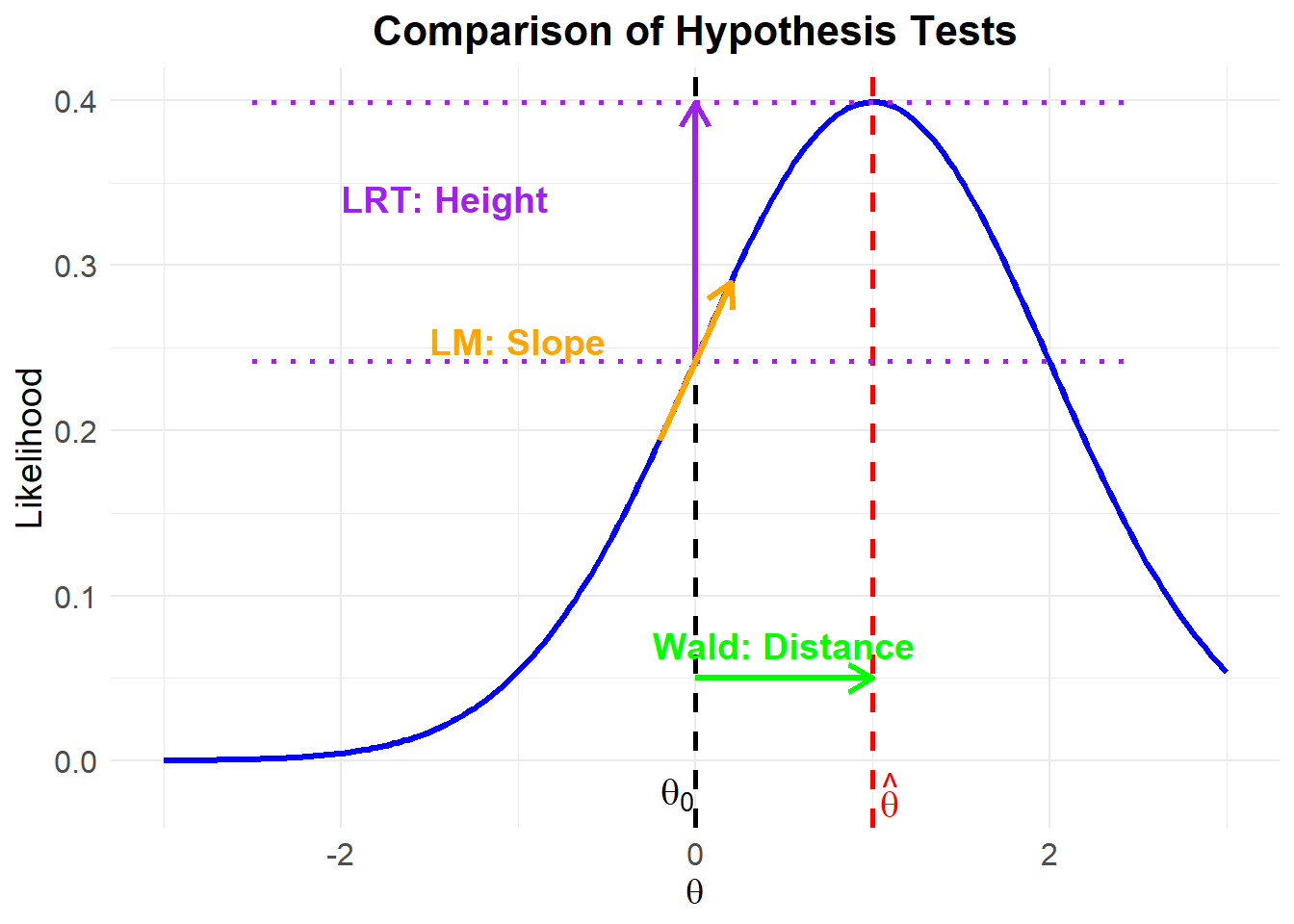
Figure 16.1: Comparison of Hypothesis Tests
Each test approaches hypothesis evaluation differently:
- Likelihood Ratio Test: Compares the heights of the log-likelihood at \(\hat{\theta}\) (full model) vs. \(\theta_0\) (restricted model).
- Wald Test: Measures the distance between \(\hat{\theta}\) and \(\theta_0\).
- Lagrange Multiplier Test: Examines the slope of the log-likelihood at \(\theta_0\) to check if movement towards \(\hat{\theta}\) significantly improves fit.
The Likelihood Ratio Test and Lagrange Multiplier Test perform well in small to moderate samples, while the Wald Test is computationally simpler as it only requires one model estimation.
| Test | Key Idea | Computation | Best Use Case |
|---|---|---|---|
| Likelihood Ratio Test | Compares log-likelihoods of full vs. restricted models | Estimates both models | When both models can be estimated |
| Wald Test | Checks if parameters significantly differ from \(H_0\) | Estimates only the full model | When the full model is available |
| Lagrange Multiplier Test | Tests if the score function suggests moving away from \(H_0\) | Estimates only the restricted model | When the full model is difficult to estimate |