6.2 Non-linear Least Squares Estimation
The least squares (LS) estimate of \(\theta\), denoted as \(\hat{\theta}\), minimizes the residual sum of squares:
\[ S(\hat{\theta}) = SSE(\hat{\theta}) = \sum_{i=1}^{n} \{Y_i - f(\mathbf{x}_i; \hat{\theta})\}^2 \]
To solve this, we consider the partial derivatives of \(S(\theta)\) with respect to each \(\theta_j\) and set them to zero, leading to the normal equations:
\[ \frac{\partial S(\theta)}{\partial \theta_j} = -2 \sum_{i=1}^{n} \{Y_i - f(\mathbf{x}_i; \theta)\} \frac{\partial f(\mathbf{x}_i; \theta)}{\partial \theta_j} = 0 \]
However, these equations are inherently non-linear and, in most cases, cannot be solved analytically. As a result, various estimation techniques are employed to approximate solutions efficiently. These approaches include:
- Iterative Optimization – Methods that refine estimates through successive iterations to minimize error.
- Derivative-Free Methods – Techniques that do not rely on gradient information, useful for complex or non-smooth functions.
- Stochastic Heuristic – Algorithms that incorporate randomness, such as genetic algorithms or simulated annealing, to explore solution spaces.
- Linearization– Approximating non-linear models with linear ones to enable analytical or numerical solutions.
- Hybrid Approaches – Combining multiple methods to leverage their respective strengths for improved estimation.
| Category | Method | Best For | Derivative? | Optimization | Comp. Cost |
|---|---|---|---|---|---|
| Iterative Optimization | Steepest Descent (Gradient Descent) | Simple problems, slow convergence | Yes | Local | Low |
| Iterative Optimization | Gauss-Newton Algorithm | Faster than GD, ignores exact second-order info | Yes | Local | Medium |
| Iterative Optimization | Levenberg-Marquardt Algorithm | Balances GN & GD, robust | Yes | Local | Medium |
| Iterative Optimization | Newton-Raphson Method | Quadratic convergence, needs Hessian | Yes | Local | High |
| Iterative Optimization | Quasi-Newton Method | Approximates Hessian for large problems | Yes | Local | Medium |
| Iterative Optimization | Trust-Region Reflective Algorithm | Handles constraints, robust | Yes | Local | High |
| Derivative-Free | Secant Method | Approximates derivative from function evaluations | No | Local | Medium |
| Derivative-Free | Nelder-Mead (Simplex) | No derivatives, heuristic | No | Local | Medium |
| Derivative-Free | Powell’s Method | Line search, no explicit gradient | No | Local | Medium |
| Derivative-Free | Grid Search | Exhaustive search (best in low dims) | No | Global | Very High |
| Derivative-Free | Hooke-Jeeves Pattern Search | Pattern-based, black-box optimization | No | Local | Medium |
| Derivative-Free | Bisection Method | Simple root/interval-based approach | No | Local | Low |
| Stochastic Heuristic | Simulated Annealing | Escapes local minima, non-smooth problems | No | Global | High |
| Stochastic Heuristic | Genetic Algorithm | Large search spaces, evolving parameters | No | Global | High |
| Stochastic Heuristic | Particle Swarm Optimization | Swarm-based, often fast global convergence | No | Global | Medium |
| Stochastic Heuristic | Evolutionary Strategies | High-dimensional, adaptive step-size | No | Global | High |
| Stochastic Heuristic | Differential Evolution Algorithm | Robust global optimizer, population-based | No | Global | High |
| Stochastic Heuristic | Ant Colony Optimization (ACO) | Discrete / combinatorial problems | No | Global | High |
| Linearization | Taylor Series Approximation | Local approximation of non-linearity | Yes | Local | Low |
| Linearization | Log-Linearization | Transforms non-linear equations | Yes | Local | Low |
| Hybrid | Adaptive Levenberg-Marquardt | Dynamically adjusts damping in LM | Yes | Local | Medium |
| Hybrid | Hybrid Genetic Algorithm & LM (GA-LM) | GA for coarse search, LM for fine-tuning | No | Hybrid | High |
| Hybrid | Neural Network-Based NLLS | Deep learning for complex non-linear least squares | No | Hybrid | Very High |
6.2.1 Iterative Optimization
6.2.1.1 Gauss-Newton Algorithm
The Gauss-Newton Algorithm is an iterative optimization method used to estimate parameters in nonlinear least squares problems. It refines parameter estimates by approximating the Hessian matrix using first-order derivatives, making it computationally efficient for many practical applications (e.g., regression models in finance and marketing analytics). The objective is to minimize the Sum of Squared Errors (SSE):
\[ SSE(\theta) = \sum_{i=1}^{n} [Y_i - f_i(\theta)]^2, \]
where \(\mathbf{Y} = [Y_1, \dots, Y_n]'\) are the observed responses, and \(f_i(\theta)\) are the model-predicted values.
Iterative Refinement via Taylor Expansion
The Gauss-Newton algorithm iteratively refines an initial estimate \(\hat{\theta}^{(0)}\) using the Taylor series expansion of \(f(\mathbf{x}_i; \theta)\) about \(\hat{\theta}^{(0)}\). We start with the observation model:
\[ Y_i = f(\mathbf{x}_i; \theta) + \epsilon_i. \]
By expanding \(f(\mathbf{x}_i; \theta)\) around \(\hat{\theta}^{(0)}\) and ignoring higher-order terms (assuming the remainder is small), we get:
\[ \begin{aligned} Y_i &\approx f(\mathbf{x}_i; \hat{\theta}^{(0)}) + \sum_{j=1}^{p} \frac{\partial f(\mathbf{x}_i; \theta)}{\partial \theta_j} \bigg|_{\theta = \hat{\theta}^{(0)}} \left(\theta_j - \hat{\theta}_j^{(0)}\right) + \epsilon_i. \end{aligned} \]
In matrix form, let
\[ \mathbf{Y} = \begin{bmatrix} Y_1 \\ \vdots \\ Y_n \end{bmatrix}, \quad \mathbf{f}(\hat{\theta}^{(0)}) = \begin{bmatrix} f(\mathbf{x}_1, \hat{\theta}^{(0)}) \\ \vdots \\ f(\mathbf{x}_n, \hat{\theta}^{(0)}) \end{bmatrix}, \]
and define the Jacobian matrix of partial derivatives
\[ \mathbf{F}(\hat{\theta}^{(0)}) = \begin{bmatrix} \frac{\partial f(\mathbf{x}_1, \theta)}{\partial \theta_1} & \cdots & \frac{\partial f(\mathbf{x}_1, \theta)}{\partial \theta_p} \\ \vdots & \ddots & \vdots \\ \frac{\partial f(\mathbf{x}_n, \theta)}{\partial \theta_1} & \cdots & \frac{\partial f(\mathbf{x}_n, \theta)}{\partial \theta_p} \end{bmatrix}_{\theta = \hat{\theta}^{(0)}}. \]
Then,
\[ \mathbf{Y} \approx \mathbf{f}(\hat{\theta}^{(0)}) + \mathbf{F}(\hat{\theta}^{(0)})(\theta - \hat{\theta}^{(0)}) + \epsilon, \]
with \(\epsilon = [\epsilon_1, \dots, \epsilon_n]'\) assumed i.i.d. with mean \(0\) and variance \(\sigma^2\).
From this linear approximation,
\[ \mathbf{Y} - \mathbf{f}(\hat{\theta}^{(0)}) \approx \mathbf{F}(\hat{\theta}^{(0)})(\theta - \hat{\theta}^{(0)}). \]
Solving for \(\theta - \hat{\theta}^{(0)}\) in the least squares sense gives the Gauss increment \(\hat{\delta}^{(1)}\), so we can update:
\[ \hat{\theta}^{(1)} = \hat{\theta}^{(0)} + \hat{\delta}^{(1)}. \]
Step-by-Step Procedure
- Initialize: Start with an initial estimate \(\hat{\theta}^{(0)}\) and set \(j = 0\).
- Compute Taylor Expansion: Calculate \(\mathbf{f}(\hat{\theta}^{(j)})\) and \(\mathbf{F}(\hat{\theta}^{(j)})\).
- Solve for Increment: Treating \(\mathbf{Y} - \mathbf{f}(\hat{\theta}^{(j)}) \approx \mathbf{F}(\hat{\theta}^{(j)}) (\theta - \hat{\theta}^{(j)})\) as a linear model, use Ordinary Least Squares to compute \(\hat{\delta}^{(j+1)}\).
- Update Parameters: Set \(\hat{\theta}^{(j+1)} = \hat{\theta}^{(j)} + \hat{\delta}^{(j+1)}\).
- Check for Convergence: If the convergence criteria are met (see below), stop; otherwise, return to Step 2.
- Estimate Variance: After convergence, we assume \(\epsilon \sim (\mathbf{0}, \sigma^2 \mathbf{I})\). The variance \(\sigma^2\) can be estimated by
\[ \hat{\sigma}^2 = \frac{1}{n-p} \left(\mathbf{Y} - \mathbf{f}(\mathbf{x}; \hat{\theta})\right)' \left(\mathbf{Y} - \mathbf{f}(\mathbf{x}; \hat{\theta})\right). \]
Convergence Criteria
Common criteria for deciding when to stop iterating include:
- Objective Function Change: \[ \frac{\left|SSE(\hat{\theta}^{(j+1)}) - SSE(\hat{\theta}^{(j)})\right|}{SSE(\hat{\theta}^{(j)})} < \gamma_1. \]
- Parameter Change: \[ \left|\hat{\theta}^{(j+1)} - \hat{\theta}^{(j)}\right| < \gamma_2. \]
- Residual Projection Criterion: The residuals satisfy convergence as defined in (D. M. Bates and Watts 1981).
Another way to see the update step is by viewing the necessary condition for a minimum: the gradient of \(SSE(\theta)\) with respect to \(\theta\) should be zero. For
\[ SSE(\theta) = \sum_{i=1}^{n} [Y_i - f_i(\theta)]^2, \]
the gradient is
\[ \frac{\partial SSE(\theta)}{\partial \theta} = 2\mathbf{F}(\theta)' \left[\mathbf{Y} - \mathbf{f}(\theta)\right]. \]
Using the Gauss-Newton update rule from iteration \(j\) to \(j+1\):
\[ \begin{aligned} \hat{\theta}^{(j+1)} &= \hat{\theta}^{(j)} + \hat{\delta}^{(j+1)} \\ &= \hat{\theta}^{(j)} + \left[\mathbf{F}(\hat{\theta}^{(j)})' \mathbf{F}(\hat{\theta}^{(j)})\right]^{-1} \mathbf{F}(\hat{\theta}^{(j)})' \left[\mathbf{Y} - \mathbf{f}(\hat{\theta}^{(j)})\right] \\ &= \hat{\theta}^{(j)} - \frac{1}{2} \left[\mathbf{F}(\hat{\theta}^{(j)})' \mathbf{F}(\hat{\theta}^{(j)})\right]^{-1} \frac{\partial SSE(\hat{\theta}^{(j)})}{\partial \theta}, \end{aligned} \]
where:
- \(\frac{\partial SSE(\hat{\theta}^{(j)})}{\partial \theta}\) is the gradient vector, pointing in the direction of steepest ascent of SSE.
- \(\left[\mathbf{F}(\hat{\theta}^{(j)})'\mathbf{F}(\hat{\theta}^{(j)})\right]^{-1}\) determines the step size, controlling how far to move in the direction of improvement.
- The factor \(-\tfrac{1}{2}\) ensures movement in the direction of steepest descent, helping to minimize the SSE.
The Gauss-Newton method works well when the nonlinear model can be approximated accurately by a first-order Taylor expansion near the solution. If the assumption of near-linearity in the residual function \(\mathbf{r}(\theta) = \mathbf{Y} - \mathbf{f}(\theta)\) is violated, convergence may be slow or fail altogether. In such cases, more robust methods like Levenberg-Marquardt Algorithm (which modifies Gauss-Newton with a damping parameter) are often preferred.
# Load necessary libraries
library(minpack.lm)  # Provides nonlinear least squares functions

# Define a nonlinear function (exponential model)
nonlinear_model <- function(theta, x) {
    # theta is a vector of parameters: theta[1] = A, theta[2] = B
    # x is the independent variable
    # The model is A * exp(B * x)
    theta[1] * exp(theta[2] * x)
}

# Define SSE function for clarity
sse <- function(theta, x, y) {
    # SSE = sum of squared errors between actual y and model predictions
    sum((y - nonlinear_model(theta, x)) ^ 2)
}

# Generate synthetic data
set.seed(123)                     # for reproducibility
x <- seq(0, 10, length.out = 100) # 100 points from 0 to 10
true_theta <- c(2, 0.3)           # true parameter values
y <- nonlinear_model(true_theta, x) + rnorm(length(x), sd = 0.5)

# Display the first few data points
head(data.frame(x, y))
#>           x        y
#> 1 0.0000000 1.719762
#> 2 0.1010101 1.946445
#> 3 0.2020202 2.904315
#> 4 0.3030303 2.225593
#> 5 0.4040404 2.322373
#> 6 0.5050505 3.184724

# Gauss-Newton optimization using nls.lm (Levenberg-Marquardt as extension).
# Initial guess for theta: c(1, 0.1)
fit <- nls.lm(
    par = c(1, 0.1),
    fn = function(theta)
        y - nonlinear_model(theta, x)
)

# Display estimated parameters
cat("Estimated parameters (A, B):\n")
#> Estimated parameters (A, B):
print(fit$par)
#> [1] 1.9934188 0.3008742- We defined the model “nonlinear_model(theta, x)” which returns Aexp(Bx).
- We generated synthetic data using the “true_theta” values and added random noise.
- We used
nls.lm(...)from theminpack.lmpackage to fit the data:par = c(1, 0.1)is our initial parameter guess.fn = function(theta) y - nonlinear_model(theta, x)is the residual function, i.e., observed minus predicted.
- The
fit$parprovides the estimated parameters after the algorithm converges.
# Visualize the data and the fitted model
plot(
  x,
  y,
  main = "Data and Fitted Curve (Gauss-Newton/Levenberg-Marquardt)",
  xlab = "x",
  ylab = "y",
  pch = 19,
  cex = 0.5
)
curve(
  nonlinear_model(fit$par, x),
  from = 0,
  to = 10,
  add = TRUE,
  col = "red",
  lwd = 2
)
legend(
  "topleft",
  legend = c("Data", "Fitted Curve"),
  pch = c(19, NA),
  lty = c(NA, 1),
  col = c("black", "red")
)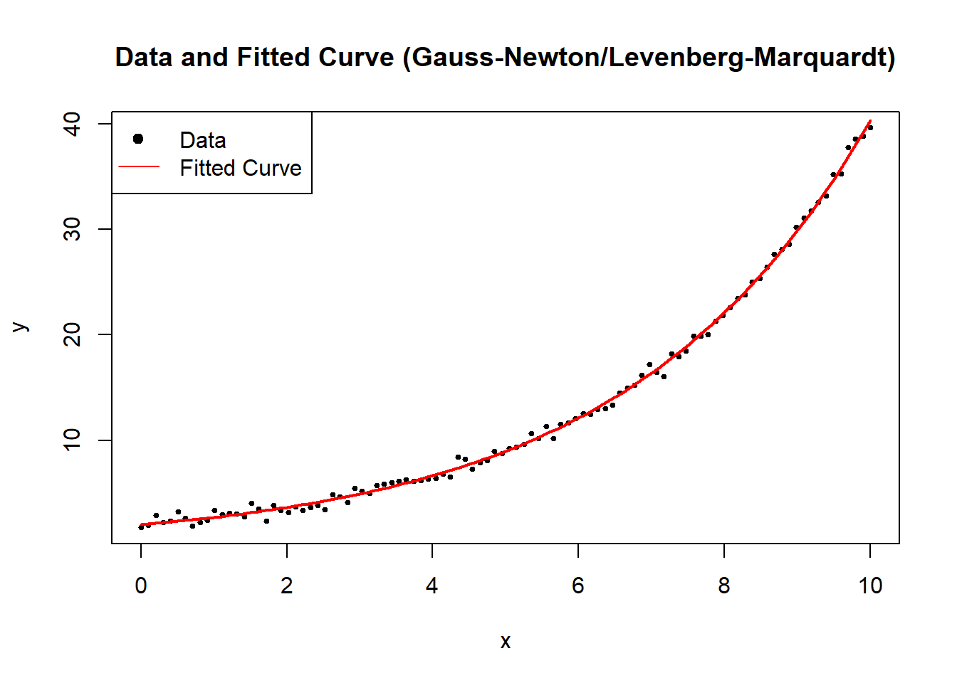
Figure 6.1: Data and Fitted Curve (Gauss–Newton/Levenberg–Marquardt)
6.2.1.2 Modified Gauss-Newton Algorithm
The Modified Gauss-Newton Algorithm introduces a learning rate \(\alpha_j\) to control step size and prevent overshooting the local minimum. The standard Gauss-Newton Algorithm assumes that the full step direction \(\hat{\delta}^{(j+1)}\) is optimal, but in practice, especially for highly nonlinear problems, it can overstep the minimum or cause numerical instability. The modification introduces a step size reduction, making it more robust.
We redefine the update step as:
\[ \hat{\theta}^{(j+1)} = \hat{\theta}^{(j)} + \alpha_j \hat{\delta}^{(j+1)}, \quad 0 < \alpha_j < 1, \]
where:
- \(\alpha_j\) is a learning rate, controlling how much of the step \(\hat{\delta}^{(j+1)}\) is taken.
- If \(\alpha_j = 1\), we recover the standard Gauss-Newton method.
- If \(\alpha_j\) is too small, convergence is slow; if too large, the algorithm may diverge.
This learning rate \(\alpha_j\) allows for adaptive step size adjustments, helping prevent excessive parameter jumps and ensuring that SSE decreases at each iteration.
A common approach to determine \(\alpha_j\) is step halving, ensuring that each iteration moves in a direction that reduces SSE. Instead of using a fixed \(\alpha_j\), we iteratively reduce the step size until SSE decreases:
\[ \hat{\theta}^{(j+1)} = \hat{\theta}^{(j)} + \frac{1}{2^k}\hat{\delta}^{(j+1)}, \]
where:
- \(k\) is the smallest non-negative integer such that
\[ SSE(\hat{\theta}^{(j)} + \frac{1}{2^k} \hat{\delta}^{(j+1)}) < SSE(\hat{\theta}^{(j)}). \]
This means we start with the full step \(\hat{\delta}^{(j+1)}\), then try \(\hat{\delta}^{(j+1)}/2\), then \(\hat{\delta}^{(j+1)}/4\), and so on, until SSE is reduced.
Algorithm for Step Halving:
- Compute the Gauss-Newton step \(\hat{\delta}^{(j+1)}\).
- Set an initial \(\alpha_j = 1\).
- If the updated parameters \(\hat{\theta}^{(j)} + \alpha_j \hat{\delta}^{(j+1)}\) increase SSE, divide \(\alpha_j\) by 2.
- Repeat until SSE decreases.
This ensures monotonic SSE reduction, preventing divergence due to an overly aggressive step.
Generalized Form of the Modified Algorithm
A more general form of the update rule, incorporating step size control and a matrix \(\mathbf{A}_j\), is:
\[ \hat{\theta}^{(j+1)} = \hat{\theta}^{(j)} - \alpha_j \mathbf{A}_j \frac{\partial Q(\hat{\theta}^{(j)})}{\partial \theta}, \]
where:
- \(\mathbf{A}_j\) is a positive definite matrix that preconditions the update direction.
- \(\alpha_j\) is the learning rate.
- \(\frac{\partial Q(\hat{\theta}^{(j)})}{\partial \theta}\) is the gradient of the objective function \(Q(\theta)\), typically SSE in nonlinear regression.
Connection to the Modified Gauss-Newton Algorithm
The Modified Gauss-Newton Algorithm fits this framework:
\[ \hat{\theta}^{(j+1)} = \hat{\theta}^{(j)} - \alpha_j [\mathbf{F}(\hat{\theta}^{(j)})' \mathbf{F}(\hat{\theta}^{(j)})]^{-1} \frac{\partial SSE(\hat{\theta}^{(j)})}{\partial \theta}. \]
Here, we recognize:
- Objective function: \(Q = SSE\).
- Preconditioner matrix: \([\mathbf{F}(\hat{\theta}^{(j)})' \mathbf{F}(\hat{\theta}^{(j)})]^{-1} = \mathbf{A}\).
Thus, the standard Gauss-Newton method can be interpreted as a special case of this broader optimization framework, with a preconditioned gradient descent approach.
# Load required library
library(minpack.lm)

# Define a nonlinear function (exponential model)
nonlinear_model <- function(theta, x) {
  theta[1] * exp(theta[2] * x)
}

# Define the Sum of Squared Errors function
sse <- function(theta, x, y) {
  sum((y - nonlinear_model(theta, x)) ^ 2)
}

# Generate synthetic data
set.seed(123)
x <- seq(0, 10, length.out = 100)
true_theta <- c(2, 0.3)
y <- nonlinear_model(true_theta, x) + rnorm(length(x), sd = 0.5)

# Gauss-Newton with Step Halving
gauss_newton_modified <-
  function(theta_init,
           x,
           y,
           tol = 1e-6,
           max_iter = 100) {
    theta <- theta_init
    for (j in 1:max_iter) {
      # Compute Jacobian matrix numerically
      epsilon <- 1e-6
      F_matrix <-
        matrix(0, nrow = length(y), ncol = length(theta))
      for (p in 1:length(theta)) {
        theta_perturb <- theta
        theta_perturb[p] <- theta[p] + epsilon
        F_matrix[, p] <-
          (nonlinear_model(theta_perturb, x)-nonlinear_model(theta, x))/epsilon
      }

      # Compute residuals
      residuals <- y - nonlinear_model(theta, x)

      # Compute Gauss-Newton step
      delta <-
        solve(t(F_matrix) %*% F_matrix) %*% t(F_matrix) %*% residuals

      # Step Halving Implementation
      alpha <- 1
      k <- 0
      while (sse(theta + alpha * delta, x, y) >= sse(theta, x, y) &&
             k < 10) {
        alpha <- alpha / 2
        k <- k + 1
      }

      # Update theta
      theta_new <- theta + alpha * delta

      # Check for convergence
      if (sum(abs(theta_new - theta)) < tol) {
        break
      }

      theta <- theta_new
    }
    return(theta)
  }

# Run Modified Gauss-Newton Algorithm
theta_init <- c(1, 0.1)  # Initial parameter guess
estimated_theta <- gauss_newton_modified(theta_init, x, y)

# Display estimated parameters
cat("Estimated parameters (A, B) with Modified Gauss-Newton:\n")
#> Estimated parameters (A, B) with Modified Gauss-Newton:
print(estimated_theta)
#>           [,1]
#> [1,] 1.9934188
#> [2,] 0.3008742
# Plot data and fitted curve
plot(
x,
y,
main = "Modified Gauss-Newton: Data & Fitted Curve",
pch = 19,
cex = 0.5,
xlab = "x",
ylab = "y"
)
curve(
nonlinear_model(estimated_theta, x),
from = 0,
to = 10,
add = TRUE,
col = "red",
lwd = 2
)
legend(
"topleft",
legend = c("Data", "Fitted Curve"),
pch = c(19, NA),
lty = c(NA, 1),
col = c("black", "red")
)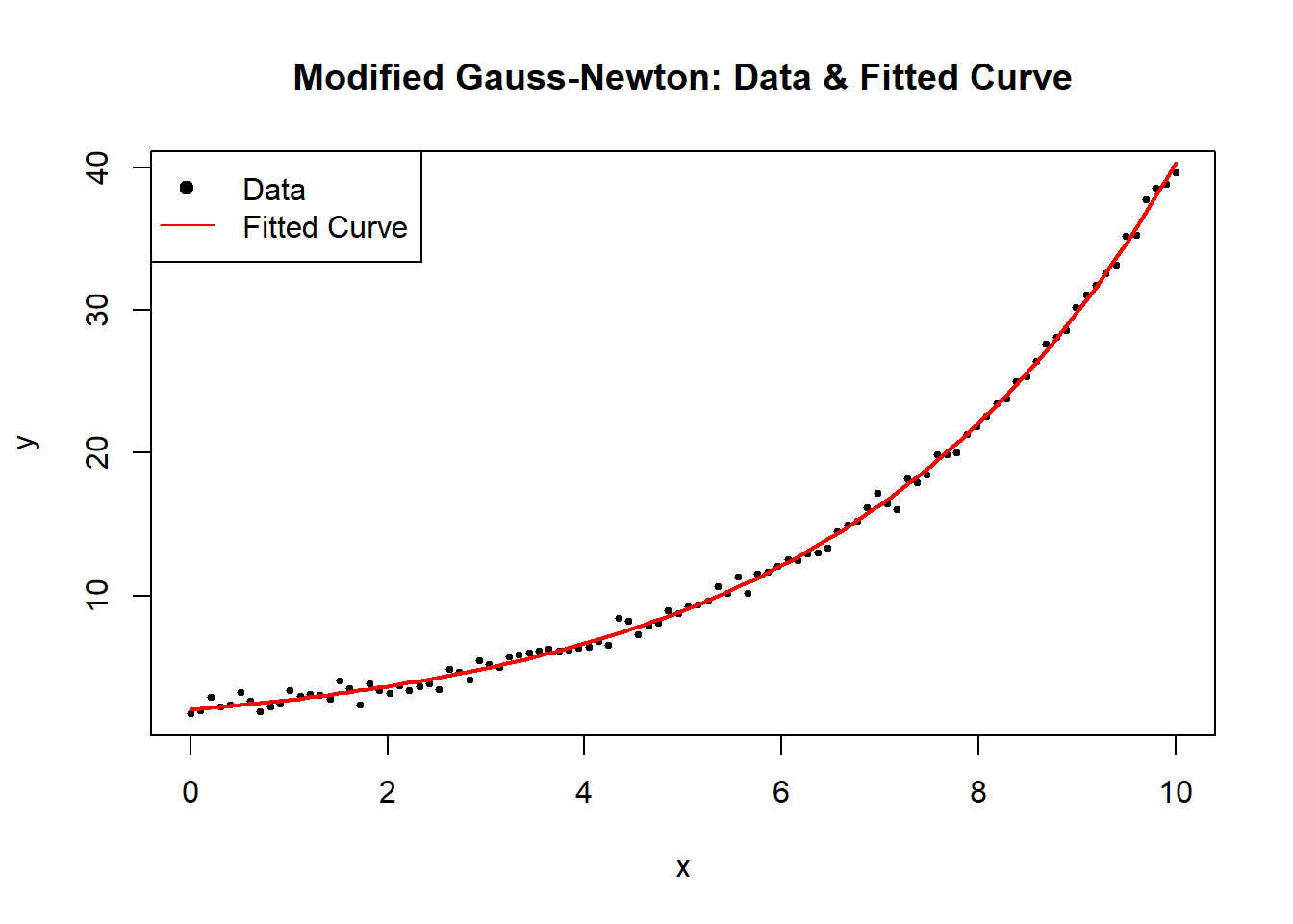
Figure 6.2: Modified Gauss–Newton
6.2.1.3 Steepest Descent (Gradient Descent)
The Steepest Descent Method, commonly known as Gradient Descent, is a fundamental iterative optimization technique used for finding parameter estimates that minimize an objective function \(\mathbf{Q}(\theta)\). It is a special case of the Modified Gauss-Newton Algorithm, where the preconditioning matrix \(\mathbf{A}_j\) is replaced by the identity matrix.
The update rule is given by:
\[ \hat{\theta}^{(j+1)} = \hat{\theta}^{(j)} - \alpha_j \mathbf{I}_{p \times p}\frac{\partial \mathbf{Q}(\hat{\theta}^{(j)})}{\partial \theta}, \]
where:
- \(\alpha_j\) is the learning rate, determining the step size.
- \(\mathbf{I}_{p \times p}\) is the identity matrix, meaning updates occur in the direction of the negative gradient.
- \(\frac{\partial \mathbf{Q}(\hat{\theta}^{(j)})}{\partial \theta}\) is the gradient vector, which provides the direction of steepest ascent; its negation ensures movement toward the minimum.
Characteristics of Steepest Descent
- Slow to converge: The algorithm moves in the direction of the gradient but does not take into account curvature, which may result in slow convergence, especially in ill-conditioned problems.
- Moves rapidly initially: The method can exhibit fast initial progress, but as it approaches the minimum, step sizes become small, leading to slow convergence.
- Useful for initialization: Due to its simplicity and ease of implementation, it is often used to obtain starting values for more advanced methods like Newton’s method or Gauss-Newton Algorithm.
| Method | Update Rule | Advantages | Disadvantages |
|---|---|---|---|
| Steepest Descent | \(\hat{\theta}^{(j+1)} = \hat{\theta}^{(j)} - \alpha_j \mathbf{I} \nabla Q(\theta)\) | Simple, requires only first derivatives | Slow convergence, sensitive to \(\alpha_j\) |
| Gauss-Newton | \(\hat{\theta}^{(j+1)} = \hat{\theta}^{(j)} - \mathbf{H}^{-1} \nabla Q(\theta)\) | Uses curvature, faster near solution | Requires Jacobian computation, may diverge |
The key difference is that Steepest Descent only considers the gradient direction, while Gauss-Newton and Newton’s method incorporate curvature information.
Choosing the Learning Rate \(\alpha_j\)
A well-chosen learning rate is crucial for the success of gradient descent:
- Too large: The algorithm may overshoot the minimum and diverge.
- Too small: Convergence is very slow.
- Adaptive strategies:
- Fixed step size: \(\alpha_j\) is constant.
- Step size decay: \(\alpha_j\) decreases over iterations (e.g., \(\alpha_j = \frac{1}{j}\)).
- Line search: Choose \(\alpha_j\) by minimizing \(\mathbf{Q}(\theta^{(j+1)})\) along the gradient direction.
A common approach is backtracking line search, where \(\alpha_j\) is reduced iteratively until a decrease in \(\mathbf{Q}(\theta)\) is observed.
# Load necessary libraries
library(ggplot2)


# Define the nonlinear function (exponential model)
nonlinear_model <- function(theta, x) {
    theta[1] * exp(theta[2] * x)
}

# Define the Sum of Squared Errors function
sse <- function(theta, x, y) {
    sum((y - nonlinear_model(theta, x)) ^ 2)
}

# Define Gradient of SSE w.r.t theta (computed numerically)
gradient_sse <- function(theta, x, y) {
    n <- length(y)
    residuals <- y - nonlinear_model(theta, x)

    # Partial derivative w.r.t theta_1
    grad_1 <- -2 * sum(residuals * exp(theta[2] * x))

    # Partial derivative w.r.t theta_2
    grad_2 <- -2 * sum(residuals * theta[1] * x * exp(theta[2] * x))

    return(c(grad_1, grad_2))
}

# Generate synthetic data
set.seed(123)
x <- seq(0, 10, length.out = 100)
true_theta <- c(2, 0.3)
y <- nonlinear_model(true_theta, x) + rnorm(length(x), sd = 0.5)

# Safe Gradient Descent Implementation
gradient_descent <-
    function(theta_init,
             x,
             y,
             alpha = 0.01,
             tol = 1e-6,
             max_iter = 500) {
        theta <- theta_init
        sse_values <- numeric(max_iter)

        for (j in 1:max_iter) {
            grad <- gradient_sse(theta, x, y)

            # Check for NaN or Inf values in the gradient (prevents divergence)
            if (any(is.na(grad)) || any(is.infinite(grad))) {
                cat("Numerical instability detected at iteration",
                    j,
                    "\n")
                break
            }

            # Update step
            theta_new <- theta - alpha * grad
            sse_values[j] <- sse(theta_new, x, y)

            # Check for convergence
            if (!is.finite(sse_values[j])) {
                cat("Divergence detected at iteration", j, "\n")
                break
            }

            if (sum(abs(theta_new - theta)) < tol) {
                cat("Converged in", j, "iterations.\n")
                return(list(theta = theta_new, sse_values = sse_values[1:j]))
            }

            theta <- theta_new
        }

        return(list(theta = theta, sse_values = sse_values))
    }

# Run Gradient Descent with a Safe Implementation
theta_init <- c(1, 0.1)  # Initial guess
alpha <- 0.001           # Learning rate
result <- gradient_descent(theta_init, x, y, alpha)
#> Divergence detected at iteration 1

# Extract results
estimated_theta <- result$theta
sse_values <- result$sse_values

# Display estimated parameters
cat("Estimated parameters (A, B) using Gradient Descent:\n")
#> Estimated parameters (A, B) using Gradient Descent:
print(estimated_theta)
#> [1] 1.0 0.1
# Plot convergence of SSE over iterations
# Ensure sse_values has valid data
sse_df <- data.frame(
Iteration = seq_along(sse_values),
SSE = sse_values
)
# Generate improved plot using ggplot()
ggplot(sse_df, aes(x = Iteration, y = SSE)) +
geom_line(color = "blue", linewidth = 1) +
labs(
title = "Gradient Descent Convergence",
x = "Iteration",
y = "SSE"
) +
theme_minimal()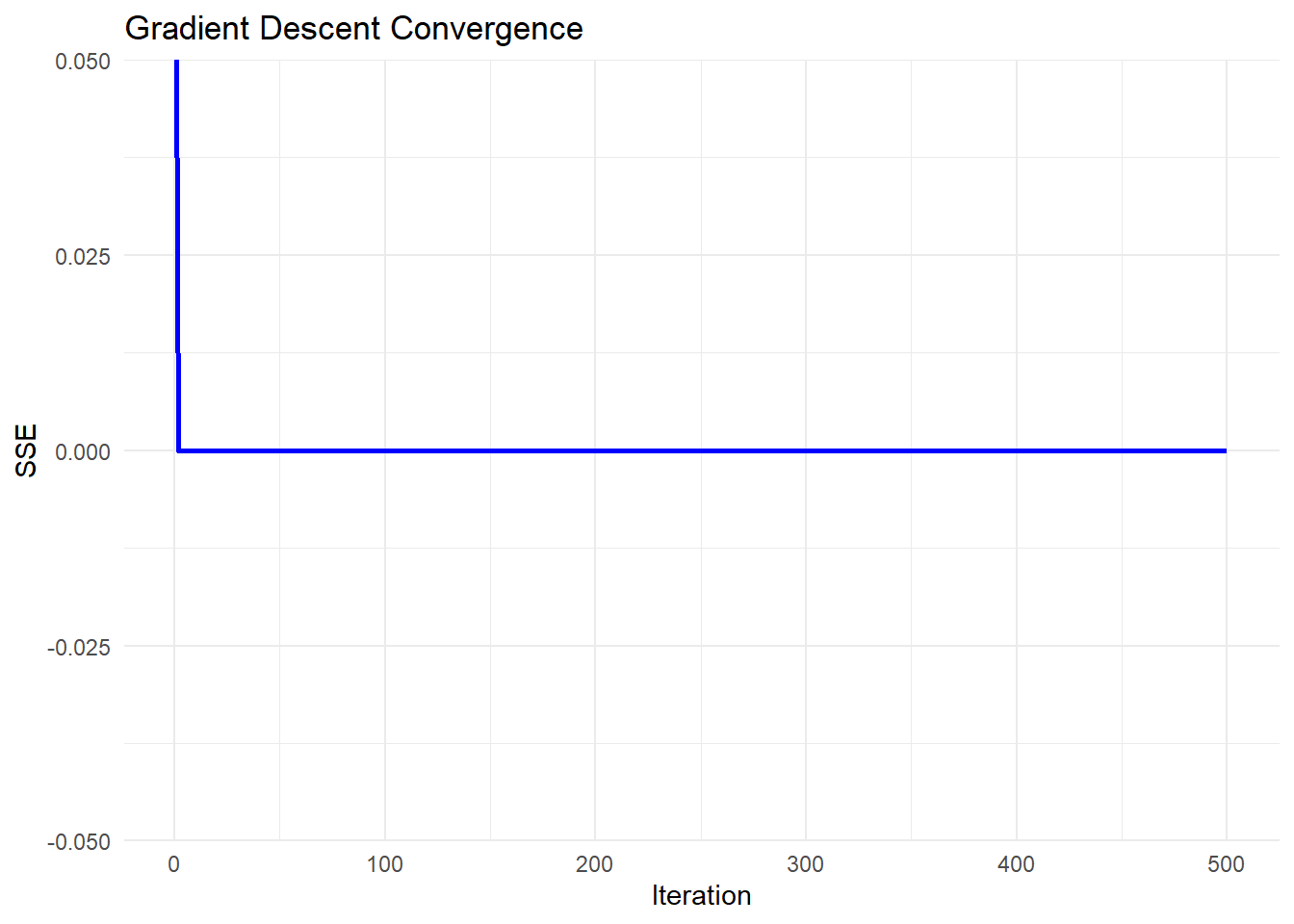
Figure 6.3: Gradient Descent Convergence
- Steepest Descent (Gradient Descent) moves in the direction of steepest descent, which can lead to zigzagging behavior.
- Slow convergence occurs when the curvature of the function varies significantly across dimensions.
- Learning rate tuning is critical:
If too large, the algorithm diverges.
If too small, progress is very slow.
- Useful for initialization: It is often used to get close to the optimal solution before switching to more advanced methods like Gauss-Newton Algorithm or Newton’s method.
Several advanced techniques improve the performance of steepest descent:
Momentum Gradient Descent: Adds a momentum term to smooth updates, reducing oscillations.
Adaptive Learning Rates:
AdaGrad: Adjusts \(\alpha_j\) per parameter based on historical gradients.
RMSprop: Uses a moving average of past gradients to scale updates.
Adam (Adaptive Moment Estimation): Combines momentum and adaptive learning rates.
In practice, Adam is widely used in machine learning and deep learning, while Newton-based methods (including Gauss-Newton) are preferred for nonlinear regression.
6.2.1.4 Levenberg-Marquardt Algorithm
The Levenberg-Marquardt Algorithm is a widely used optimization method for solving nonlinear least squares problems. It is an adaptive technique that blends the Gauss-Newton Algorithm and Steepest Descent (Gradient Descent), dynamically switching between them based on problem conditions.
The update rule is:
\[ \hat{\theta}^{(j+1)} = \hat{\theta}^{(j)} - \alpha_j [\mathbf{F}(\hat{\theta}^{(j)})' \mathbf{F}(\hat{\theta}^{(j)}) + \tau \mathbf{I}_{p \times p}]\frac{\partial \mathbf{Q}(\hat{\theta}^{(j)})}{\partial \theta} \]
where:
- \(\tau\) is the damping parameter, controlling whether the step behaves like Gauss-Newton Algorithm or Steepest Descent (Gradient Descent).
- \(\mathbf{I}_{p \times p}\) is the identity matrix, ensuring numerical stability.
- \(\mathbf{F}(\hat{\theta}^{(j)})\) is the Jacobian matrix of partial derivatives.
- \(\frac{\partial \mathbf{Q}(\hat{\theta}^{(j)})}{\partial \theta}\) is the gradient vector.
- \(\alpha_j\) is the learning rate, determining step size.
The Levenberg-Marquardt algorithm is particularly useful when the Jacobian matrix \(\mathbf{F}(\hat{\theta}^{(j)})\) is nearly singular, meaning that Gauss-Newton Algorithm alone may fail.
- When \(\tau\) is large, the method behaves like Steepest Descent, ensuring stability.
- When \(\tau\) is small, it behaves like Gauss-Newton, accelerating convergence.
- Adaptive control of \(\tau\):
- If \(SSE(\hat{\theta}^{(j+1)}) < SSE(\hat{\theta}^{(j)})\), reduce \(\tau\): \[ \tau \gets \tau / 10 \]
- Otherwise, increase \(\tau\) to stabilize: \[ \tau \gets 10\tau \]
This adjustment ensures that the algorithm moves efficiently while avoiding instability.
# Load required libraries
library(minpack.lm)
library(ggplot2)

# Define a nonlinear function (exponential model)
nonlinear_model <- function(theta, x) {
    theta[1] * exp(theta[2] * x)
}

# Define SSE function
sse <- function(theta, x, y) {
    sum((y - nonlinear_model(theta, x)) ^ 2)
}

# Generate synthetic data
set.seed(123)
x <- seq(0, 10, length.out = 100)
true_theta <- c(2, 0.3)
y <- nonlinear_model(true_theta, x) + rnorm(length(x), sd = 0.5)

# Robust Levenberg-Marquardt Optimization Implementation
levenberg_marquardt <-
    function(theta_init,
             x,
             y,
             tol = 1e-6,
             max_iter = 500,
             tau_init = 1) {
        theta <- theta_init
        tau <- tau_init
        lambda <- 1e-8  # Small regularization term
        sse_values <- numeric(max_iter)

        for (j in 1:max_iter) {
            # Compute Jacobian matrix numerically
            epsilon <- 1e-6
            F_matrix <-
                matrix(0, nrow = length(y), ncol = length(theta))
            for (p in 1:length(theta)) {
                theta_perturb <- theta
                theta_perturb[p] <- theta[p] + epsilon
                F_matrix[, p] <-
                    (nonlinear_model(theta_perturb, x)
                     - nonlinear_model(theta, x)) / epsilon
            }

            # Compute residuals
            residuals <- y - nonlinear_model(theta, x)

            # Compute Levenberg-Marquardt update
            A <-
                t(F_matrix) %*% F_matrix + tau * diag(length(theta))
            + lambda * diag(length(theta))  # Regularized A
            delta <- tryCatch(
                solve(A) %*% t(F_matrix) %*% residuals,
                error = function(e) {
                    cat("Singular matrix detected at iteration",
                        j,
                        "- Increasing tau\n")
                    tau <<- tau * 10  # Increase tau to stabilize
                    # Return zero delta to avoid NaN updates
                    return(rep(0, length(theta)))
                }
            )

            theta_new <- theta + delta

            # Compute new SSE
            sse_values[j] <- sse(theta_new, x, y)

            # Adjust tau dynamically
            if (sse_values[j] < sse(theta, x, y)) {
                # Reduce tau but prevent it from going too low
                tau <-
                    max(tau / 10, 1e-8)
            } else {
                tau <- tau * 10  # Increase tau if SSE increases
            }

            # Check for convergence
            if (sum(abs(delta)) < tol) {
                cat("Converged in", j, "iterations.\n")
                return(list(theta = theta_new, sse_values = sse_values[1:j]))
            }

            theta <- theta_new
        }

        return(list(theta = theta, sse_values = sse_values))
    }

# Run Levenberg-Marquardt
theta_init <- c(1, 0.1)  # Initial guess
result <- levenberg_marquardt(theta_init, x, y)
#> Singular matrix detected at iteration 11 - Increasing tau
#> Converged in 11 iterations.

# Extract results
estimated_theta <- result$theta
sse_values <- result$sse_values

# Display estimated parameters
cat("Estimated parameters (A, B) using Levenberg-Marquardt:\n")
#> Estimated parameters (A, B) using Levenberg-Marquardt:
print(estimated_theta)
#>               [,1]
#> [1,] -6.473440e-09
#> [2,]  1.120637e+01
# Plot convergence of SSE over iterations
sse_df <-
data.frame(Iteration = seq_along(sse_values), SSE = sse_values)
ggplot(sse_df, aes(x = Iteration, y = SSE)) +
geom_line(color = "blue", linewidth = 1) +
labs(title = "Levenberg-Marquardt Convergence",
x = "Iteration",
y = "SSE") +
theme_minimal()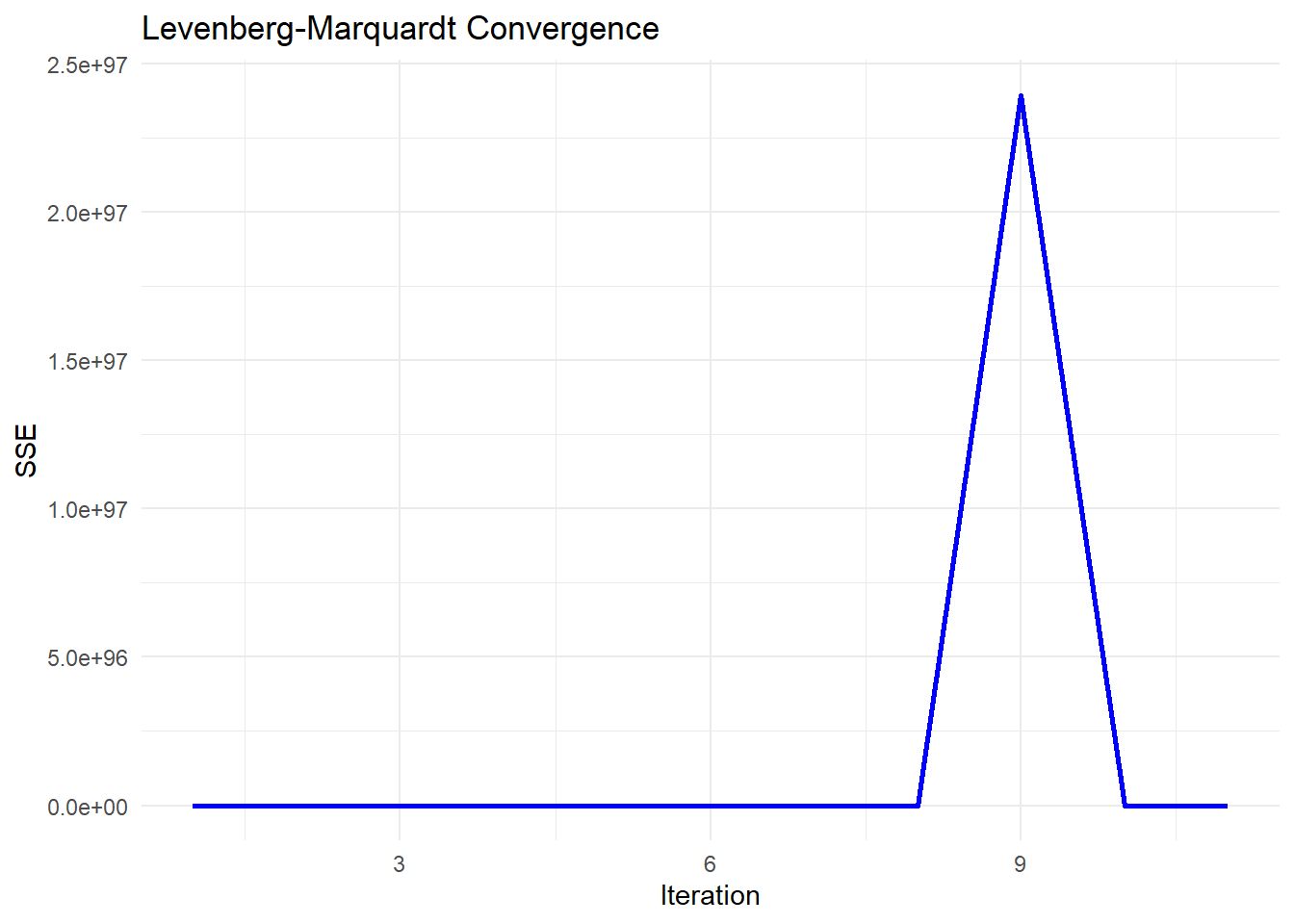
Figure 6.4: Levenberg–Marquardt Convergence
Early Stability (Flat SSE)
The SSE remains near zero for the first few iterations, which suggests that the algorithm is initially behaving stably.
This might indicate that the initial parameter guess is reasonable, or that the updates are too small to significantly affect SSE.
Sudden Explosion in SSE (Iteration ~8-9)
The sharp spike in SSE at iteration 9 indicates a numerical instability or divergence in the optimization process.
This could be due to:
An ill-conditioned Jacobian matrix: The step direction is poorly estimated, leading to an unstable jump.
A sudden large update (
delta): The damping parameter (tau) might have been reduced too aggressively, causing an uncontrolled step.Floating-point issues: If
Abecomes nearly singular, solvingA \ delta = residualsmay produce excessively large values.
Return to Stability (After Iteration 9)
The SSE immediately returns to a low value after the spike, which suggests that the damping parameter (
tau) might have been increased after detecting instability.This is consistent with the adaptive nature of Levenberg-Marquardt:
If a step leads to a bad SSE increase, the algorithm increases
tauto make the next step more conservative.If the next step stabilizes,
taumay be reduced again.
6.2.1.5 Newton-Raphson Algorithm
The Newton-Raphson method is a second-order optimization technique used for nonlinear least squares problems. Unlike first-order methods (such as Steepest Descent (Gradient Descent) and Gauss-Newton Algorithm), Newton-Raphson uses both first and second derivatives of the objective function for faster convergence.
The update rule is:
\[ \hat{\theta}^{(j+1)} = \hat{\theta}^{(j)} - \alpha_j \left[\frac{\partial^2 Q(\hat{\theta}^{(j)})}{\partial \theta \partial \theta'}\right]^{-1} \frac{\partial Q(\hat{\theta}^{(j)})}{\partial \theta} \]
where:
- \(\frac{\partial Q(\hat{\theta}^{(j)})}{\partial \theta}\) is the gradient vector (first derivative of the objective function).
- \(\frac{\partial^2 Q(\hat{\theta}^{(j)})}{\partial \theta \partial \theta'}\) is the Hessian matrix (second derivative of the objective function).
- \(\alpha_j\) is the learning rate, controlling step size.
The Hessian matrix in nonlinear least squares problems is:
\[ \frac{\partial^2 Q(\hat{\theta}^{(j)})}{\partial \theta \partial \theta'} = 2 \mathbf{F}(\hat{\theta}^{(j)})' \mathbf{F}(\hat{\theta}^{(j)}) - 2\sum_{i=1}^{n} [Y_i - f(x_i;\theta)] \frac{\partial^2 f(x_i;\theta)}{\partial \theta \partial \theta'} \]
where:
- The first term \(2 \mathbf{F}(\hat{\theta}^{(j)})' \mathbf{F}(\hat{\theta}^{(j)})\) is the same as in the Gauss-Newton Algorithm.
- The second term \(-2\sum_{i=1}^{n} [Y_i - f(x_i;\theta)] \frac{\partial^2 f(x_i;\theta)}{\partial \theta \partial \theta'}\) contains second-order derivatives.
Key Observations
- Gauss-Newton vs. Newton-Raphson:
- Gauss-Newton approximates the Hessian by ignoring the second term.
- Newton-Raphson explicitly incorporates second-order derivatives, making it more precise but computationally expensive.
- Challenges:
- The Hessian matrix may be singular, making it impossible to invert.
- Computing second derivatives is often difficult for complex functions.
# Load required libraries
library(ggplot2)

# Define a nonlinear function (exponential model)
nonlinear_model <- function(theta, x) {
    theta[1] * exp(theta[2] * x)
}

# Define SSE function
sse <- function(theta, x, y) {
    sum((y - nonlinear_model(theta, x)) ^ 2)
}

# Compute Gradient (First Derivative) of SSE
gradient_sse <- function(theta, x, y) {
    residuals <- y - nonlinear_model(theta, x)

    # Partial derivative w.r.t theta_1
    grad_1 <- -2 * sum(residuals * exp(theta[2] * x))

    # Partial derivative w.r.t theta_2
    grad_2 <- -2 * sum(residuals * theta[1] * x * exp(theta[2] * x))

    return(c(grad_1, grad_2))
}

# Compute Hessian (Second Derivative) of SSE
hessian_sse <- function(theta, x, y) {
    residuals <- y - nonlinear_model(theta, x)

    # Compute second derivatives
    H_11 <- 2 * sum(exp(2 * theta[2] * x))
    H_12 <- 2 * sum(x * exp(2 * theta[2] * x) * theta[1])
    H_21 <- H_12

    term1 <- 2 * sum((x ^ 2) * exp(2 * theta[2] * x) * theta[1] ^ 2)
    term2 <- 2 * sum(residuals * (x ^ 2) * exp(theta[2] * x))

    H_22 <- term1 - term2

    return(matrix(
        c(H_11, H_12, H_21, H_22),
        nrow = 2,
        byrow = TRUE
    ))
}

# Generate synthetic data
set.seed(123)
x <- seq(0, 10, length.out = 100)
true_theta <- c(2, 0.3)
y <- nonlinear_model(true_theta, x) + rnorm(length(x), sd = 0.5)

# Newton-Raphson Optimization Implementation
newton_raphson <-
    function(theta_init,
             x,
             y,
             tol = 1e-6,
             max_iter = 500) {
        theta <- theta_init
        sse_values <- numeric(max_iter)

        for (j in 1:max_iter) {
            grad <- gradient_sse(theta, x, y)
            hessian <- hessian_sse(theta, x, y)

            # Check if Hessian is invertible
            if (det(hessian) == 0) {
                cat("Hessian is singular at iteration",
                    j,
                    "- Using identity matrix instead.\n")
                # Replace with identity matrix if singular
                hessian <-
                    diag(length(theta))
            }

            # Compute Newton update
            delta <- solve(hessian) %*% grad
            theta_new <- theta - delta
            sse_values[j] <- sse(theta_new, x, y)

            # Check for convergence
            if (sum(abs(delta)) < tol) {
                cat("Converged in", j, "iterations.\n")
                return(list(theta = theta_new, sse_values = sse_values[1:j]))
            }

            theta <- theta_new
        }

        return(list(theta = theta, sse_values = sse_values))
    }

# Run Newton-Raphson
theta_init <- c(1, 0.1)  # Initial guess
result <- newton_raphson(theta_init, x, y)
#> Converged in 222 iterations.

# Extract results
estimated_theta <- result$theta
sse_values <- result$sse_values

# Display estimated parameters
cat("Estimated parameters (A, B) using Newton-Raphson:\n")
#> Estimated parameters (A, B) using Newton-Raphson:
print(estimated_theta)
#>           [,1]
#> [1,] 1.9934188
#> [2,] 0.3008742
# Plot convergence of SSE over iterations
sse_df <-
data.frame(Iteration = seq_along(sse_values), SSE = sse_values)
ggplot(sse_df, aes(x = Iteration, y = SSE)) +
geom_line(color = "blue", size = 1) +
labs(title = "Newton-Raphson Convergence",
x = "Iteration",
y = "SSE") +
theme_minimal()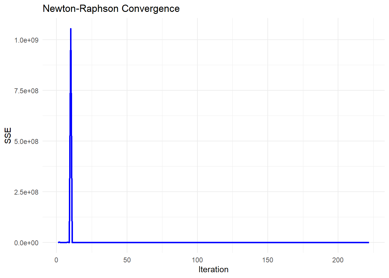
Figure 6.5: Newton–Raphson Convergence
6.2.1.6 Quasi-Newton Method
The Quasi-Newton method is an optimization technique that approximates Newton’s method without requiring explicit computation of the Hessian matrix. Instead, it iteratively constructs an approximation \(\mathbf{H}_j\) to the Hessian based on the first derivative information.
The update rule is:
\[ \hat{\theta}^{(j+1)} = \hat{\theta}^{(j)} - \alpha_j \mathbf{H}_j^{-1}\frac{\partial \mathbf{Q}(\hat{\theta}^{(j)})}{\partial \theta} \]
where:
- \(\mathbf{H}_j\) is a symmetric positive definite approximation to the Hessian matrix.
- As \(j \to \infty\), \(\mathbf{H}_j\) gets closer to the true Hessian.
- \(\frac{\partial Q(\hat{\theta}^{(j)})}{\partial \theta}\) is the gradient vector.
- \(\alpha_j\) is the learning rate, controlling step size.
Why Use Quasi-Newton Instead of Newton-Raphson Method?
- Newton-Raphson requires computing the Hessian matrix explicitly, which is computationally expensive and may be singular.
- Quasi-Newton avoids computing the Hessian directly by approximating it iteratively.
- Among first-order methods (which only require gradients, not Hessians), Quasi-Newton methods perform best.
Hessian Approximation
Instead of directly computing the Hessian \(\mathbf{H}_j\), Quasi-Newton methods update an approximation \(\mathbf{H}_j\) iteratively.
One of the most widely used formulas is the Broyden-Fletcher-Goldfarb-Shanno (BFGS) update:
\[ \mathbf{H}_{j+1} = \mathbf{H}_j + \frac{(\mathbf{s}_j \mathbf{s}_j')}{\mathbf{s}_j' \mathbf{y}_j} - \frac{\mathbf{H}_j \mathbf{y}_j \mathbf{y}_j' \mathbf{H}_j}{\mathbf{y}_j' \mathbf{H}_j \mathbf{y}_j} \]
where:
- \(\mathbf{s}_j = \hat{\theta}^{(j+1)} - \hat{\theta}^{(j)}\) (change in parameters).
- \(\mathbf{y}_j = \nabla Q(\hat{\theta}^{(j+1)}) - \nabla Q(\hat{\theta}^{(j)})\) (change in gradient).
- \(\mathbf{H}_j\) is the current inverse Hessian approximation.
# Load required libraries
library(ggplot2)

# Define a nonlinear function (exponential model)
nonlinear_model <- function(theta, x) {
    theta[1] * exp(theta[2] * x)
}

# Define SSE function
sse <- function(theta, x, y) {
    sum((y - nonlinear_model(theta, x))^2)
}

# Generate synthetic data
set.seed(123)
x <- seq(0, 10, length.out = 100)
true_theta <- c(2, 0.3)
y <- nonlinear_model(true_theta, x) + rnorm(length(x), sd = 0.5)

# Run BFGS Optimization using `optim()`
theta_init <- c(1, 0.1)  # Initial guess
result <- optim(
    par = theta_init,
    fn = function(theta) sse(theta, x, y),  # Minimize SSE
    method = "BFGS",
    control = list(trace = 0)  # Suppress optimization progress
    # control = list(trace = 1, REPORT = 1)  # Print optimization progress
)

# Extract results
estimated_theta <- result$par
sse_final <- result$value
convergence_status <- result$convergence  # 0 means successful convergence

# Display estimated parameters
cat("\n=== Optimization Results ===\n")
#>
#> === Optimization Results ===
cat("Estimated parameters (A, B) using Quasi-Newton BFGS:\n")
#> Estimated parameters (A, B) using Quasi-Newton BFGS:
print(estimated_theta)
#> [1] 1.9954216 0.3007569

# Display final SSE
cat("\nFinal SSE:", sse_final, "\n")
#>
#> Final SSE: 20.3227
6.2.1.7 Trust-Region Reflective Algorithm
The Trust-Region Reflective (TRR) algorithm is an optimization technique used for nonlinear least squares problems. Unlike Newton’s method and gradient-based approaches, TRR dynamically restricts updates to a trust region, ensuring stability and preventing overshooting.
The goal is to minimize the objective function \(Q(\theta)\) (e.g., Sum of Squared Errors, SSE):
\[ \hat{\theta} = \arg\min_{\theta} Q(\theta) \]
Instead of taking a full Newton step, TRR solves the following quadratic subproblem:
\[ \min_{\delta} m_j(\delta) = Q(\hat{\theta}^{(j)}) + \nabla Q(\hat{\theta}^{(j)})' \delta + \frac{1}{2} \delta' \mathbf{H}_j \delta \]
subject to:
\[ \|\delta\| \leq \Delta_j \]
where:
\(\mathbf{H}_j\) is an approximation of the Hessian matrix.
\(\nabla Q(\hat{\theta}^{(j)})\) is the gradient vector.
\(\Delta_j\) is the trust-region radius, which is adjusted dynamically.
Trust-Region Adjustments
The algorithm modifies the step size dynamically based on the ratio \(\rho_j\):
\[ \rho_j = \frac{Q(\hat{\theta}^{(j)}) - Q(\hat{\theta}^{(j)} + \delta)}{m_j(0) - m_j(\delta)} \]
If \(\rho_j > 0.75\) and \(\|\delta\| = \Delta_j\), then expand the trust region: \[ \Delta_{j+1} = 2 \Delta_j \]
If \(\rho_j < 0.25\), shrink the trust region: \[ \Delta_{j+1} = \frac{1}{2} \Delta_j \]
If \(\rho_j > 0\), accept the step; otherwise, reject it.
If a step violates a constraint, it is reflected back into the feasible region:
\[ \hat{\theta}^{(j+1)} = \max(\hat{\theta}^{(j)} + \delta, \theta_{\min}) \]
This ensures that the optimization respects parameter bounds.
# Load required libraries
library(ggplot2)


# Define a nonlinear function (exponential model)
nonlinear_model <- function(theta, x) {
    theta[1] * exp(theta[2] * x)
}

# Define SSE function
sse <- function(theta, x, y) {
    sum((y - nonlinear_model(theta, x)) ^ 2)
}

# Compute Gradient (First Derivative) of SSE
gradient_sse <- function(theta, x, y) {
    residuals <- y - nonlinear_model(theta, x)

    # Partial derivative w.r.t theta_1
    grad_1 <- -2 * sum(residuals * exp(theta[2] * x))

    # Partial derivative w.r.t theta_2
    grad_2 <- -2 * sum(residuals * theta[1] * x * exp(theta[2] * x))

    return(c(grad_1, grad_2))
}

# Compute Hessian Approximation of SSE
hessian_sse <- function(theta, x, y) {
    residuals <- y - nonlinear_model(theta, x)

    # Compute second derivatives
    H_11 <- 2 * sum(exp(2 * theta[2] * x))
    H_12 <- 2 * sum(x * exp(2 * theta[2] * x) * theta[1])
    H_21 <- H_12

    term1 <- 2 * sum((x ^ 2) * exp(2 * theta[2] * x) * theta[1] ^ 2)
    term2 <- 2 * sum(residuals * (x ^ 2) * exp(theta[2] * x))

    H_22 <- term1 - term2

    return(matrix(
        c(H_11, H_12, H_21, H_22),
        nrow = 2,
        byrow = TRUE
    ))
}

# Generate synthetic data
set.seed(123)
x <- seq(0, 10, length.out = 100)
true_theta <- c(2, 0.3)
y <- nonlinear_model(true_theta, x) + rnorm(length(x), sd = 0.5)

# Manual Trust-Region Reflective Optimization Implementation
trust_region_reflective <-
    function(theta_init,
             x,
             y,
             tol = 1e-6,
             max_iter = 500,
             delta_max = 1.0) {
        theta <- theta_init
        delta_j <- 0.5  # Initial trust-region size
        n <- length(theta)
        sse_values <- numeric(max_iter)

        for (j in 1:max_iter) {
            grad <- gradient_sse(theta, x, y)
            hessian <- hessian_sse(theta, x, y)

            # Check if Hessian is invertible
            if (det(hessian) == 0) {
                cat("Hessian is singular at iteration",
                    j,
                    "- Using identity matrix instead.\n")
                hessian <-
                    diag(n)  # Replace with identity matrix if singular
            }

            # Compute Newton step
            delta_full <- -solve(hessian) %*% grad

            # Apply trust-region constraint
            if (sqrt(sum(delta_full ^ 2)) > delta_j) {
                # Scale step
                delta <-
                    (delta_j / sqrt(sum(delta_full ^ 2))) * delta_full
            } else {
                delta <- delta_full
            }

            # Compute new theta and ensure it respects constraints
            theta_new <-
                pmax(theta + delta, c(0,-Inf))  # Reflect to lower bound
            sse_new <- sse(theta_new, x, y)

            # Compute agreement ratio (rho_j)
            predicted_reduction <-
                -t(grad) %*% delta - 0.5 * t(delta) %*% hessian %*% delta
            actual_reduction <- sse(theta, x, y) - sse_new
            rho_j <- actual_reduction / predicted_reduction

            # Adjust trust region size
            if (rho_j < 0.25) {
                delta_j <- max(delta_j / 2, 1e-4)  # Shrink
            } else if (rho_j > 0.75 &&
                       sqrt(sum(delta ^ 2)) == delta_j) {
                delta_j <- min(2 * delta_j, delta_max)  # Expand
            }

            # Accept or reject step
            if (rho_j > 0) {
                theta <- theta_new  # Accept step
            } else {
                cat("Step rejected at iteration", j, "\n")
            }

            sse_values[j] <- sse(theta, x, y)

            # Check for convergence
            if (sum(abs(delta)) < tol) {
                cat("Converged in", j, "iterations.\n")
                return(list(theta = theta, sse_values = sse_values[1:j]))
            }
        }

        return(list(theta = theta, sse_values = sse_values))
    }

# Run Manual Trust-Region Reflective Algorithm
theta_init <- c(1, 0.1)  # Initial guess
result <- trust_region_reflective(theta_init, x, y)

# Extract results
estimated_theta <- result$theta
sse_values <- result$sse_values
# Plot convergence of SSE over iterations
sse_df <-
data.frame(Iteration = seq_along(sse_values), SSE = sse_values)
ggplot(sse_df, aes(x = Iteration, y = SSE)) +
geom_line(color = "blue", size = 1) +
labs(title = "Trust-Region Reflective Convergence",
x = "Iteration",
y = "SSE") +
theme_minimal()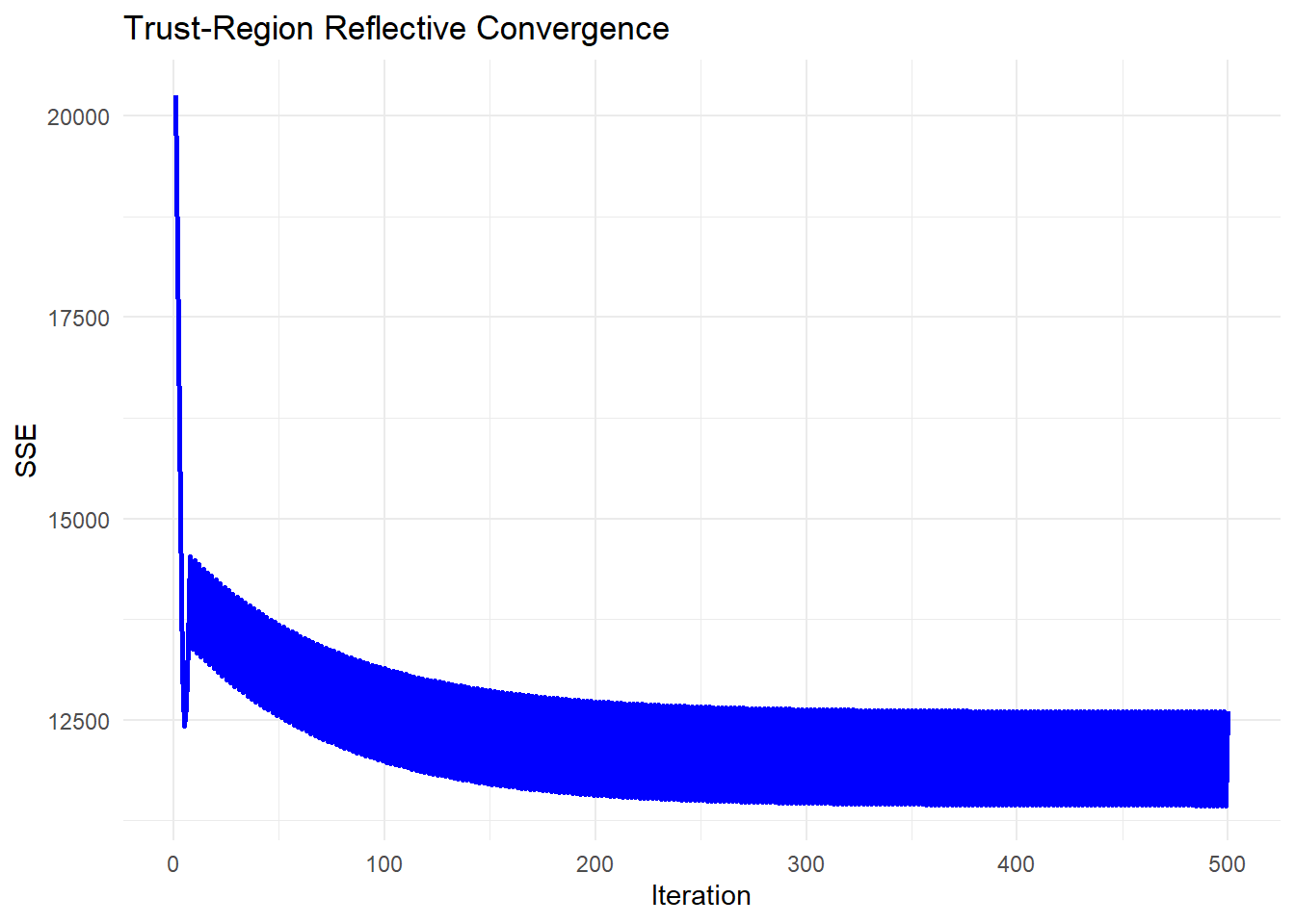
Figure 6.6: Trust-Region Reflective Convergence
6.2.2 Derivative-Free
6.2.2.1 Secant Method
The Secant Method is a root-finding algorithm that approximates the derivative using finite differences, making it a derivative-free alternative to Newton’s method. It is particularly useful when the exact gradient (or Jacobian in the case of optimization problems) is unavailable or expensive to compute.
In nonlinear optimization, we apply the Secant Method to iteratively refine parameter estimates without explicitly computing second-order derivatives.
In one dimension, the Secant Method approximates the derivative as:
\[ f'(\theta) \approx \frac{f(\theta_{j}) - f(\theta_{j-1})}{\theta_{j} - \theta_{j-1}}. \]
Using this approximation, the update step in the Secant Method follows:
\[ \theta_{j+1} = \theta_j - f(\theta_j) \frac{\theta_j - \theta_{j-1}}{f(\theta_j) - f(\theta_{j-1})}. \]
Instead of computing the exact derivative (as in Newton’s method), we use the difference between the last two iterates to approximate it. This makes the Secant Method more efficient in cases where gradient computation is expensive or infeasible.
In higher dimensions, the Secant Method extends to an approximate Quasi-Newton Method, often referred to as Broyden’s Method. We iteratively approximate the inverse Hessian matrix using past updates.
The update formula for a vector-valued function \(F(\theta)\) is:
\[ \theta^{(j+1)} = \theta^{(j)} - \mathbf{B}^{(j)} F(\theta^{(j)}), \]
where \(\mathbf{B}^{(j)}\) is an approximation of the inverse Jacobian matrix, updated at each step using:
\[ \mathbf{B}^{(j+1)} = \mathbf{B}^{(j)} + \frac{(\Delta \theta^{(j)} - \mathbf{B}^{(j)} \Delta F^{(j)}) (\Delta \theta^{(j)})'}{(\Delta \theta^{(j)})' \Delta F^{(j)}}, \]
where:
- \(\Delta \theta^{(j)} = \theta^{(j+1)} - \theta^{(j)}\),
- \(\Delta F^{(j)} = F(\theta^{(j+1)}) - F(\theta^{(j)})\).
This secant-based update approximates the behavior of the true Jacobian inverse, reducing computational cost compared to full Newton’s method.
Algorithm: Secant Method for Nonlinear Optimization
The Secant Method for nonlinear optimization follows these steps:
- Initialize parameters \(\theta^{(0)}\) and \(\theta^{(1)}\) (two starting points).
- Compute the function values \(F(\theta^{(0)})\) and \(F(\theta^{(1)})\).
- Use the Secant update formula to compute the next iterate \(\theta^{(j+1)}\).
- Update the approximate inverse Jacobian \(\mathbf{B}^{(j)}\).
- Repeat until convergence.
# Load required libraries
library(numDeriv)


# Define a nonlinear function (logistic model)
nonlinear_model <- function(theta, x) {
    return(theta[1] / (1 + exp(-theta[2] * (x - theta[3]))))
}

# Define the Sum of Squared Errors (SSE) function
sse <- function(theta, x, y) {
    return(sum((y - nonlinear_model(theta, x)) ^ 2))
}

# Generate synthetic data
set.seed(123)
x <- seq(-5, 5, length.out = 100)
true_theta <- c(4, 1.5, 0)  # True parameters (A, B, C)
y <- nonlinear_model(true_theta, x) + rnorm(length(x), sd = 0.3)

# Improved Secant Method with Line Search
secant_method_improved <-
    function(theta0,
             theta1,
             x,
             y,
             tol = 1e-6,
             max_iter = 100) {
        theta_prev <- as.matrix(theta0)  # Convert to column vector
        theta_curr <- as.matrix(theta1)

        alpha <- 1  # Initial step size
        step_reduction_factor <- 0.5  # Reduce step if SSE increases
        B_inv <- diag(length(theta0))  # Identity matrix initialization

        for (j in 1:max_iter) {
            # Compute function values using numerical gradient
            F_prev <-
                as.matrix(grad(function(theta)
                    sse(theta, x, y), theta_prev))
            F_curr <-
                as.matrix(grad(function(theta)
                    sse(theta, x, y), theta_curr))

            # Compute secant step update (convert to column vectors)
            delta_theta <- as.matrix(theta_curr - theta_prev)
            delta_F <- as.matrix(F_curr - F_prev)

            # Prevent division by zero
            if (sum(abs(delta_F)) < 1e-8) {
                cat("Gradient diff is too small, stopping optimization.\n")
                break
            }

            # Ensure correct dimensions for Broyden update
            numerator <-
                (delta_theta - B_inv %*% delta_F) %*% t(delta_theta)
            # Convert scalar to numeric
            denominator <-
                as.numeric(t(delta_theta) %*% delta_F)

            # Updated inverse Jacobian approximation
            B_inv <-
                B_inv + numerator / denominator

            # Compute next theta using secant update
            theta_next <- theta_curr - alpha * B_inv %*% F_curr

            # Line search: Reduce step size if SSE increases
            while (sse(as.vector(theta_next), x, y) > sse(as.vector(theta_curr),
                                                          x, y)) {
                alpha <- alpha * step_reduction_factor
                theta_next <- theta_curr - alpha * B_inv %*% F_curr

                # Print progress
                # cat("Reducing step size to", alpha, "\n")
            }

            # Print intermediate results for debugging
            cat(
                sprintf(
                    "Iteration %d: Theta = (%.4f, %.4f, %.4f), Alpha = %.4f\n",
                    j,
                    theta_next[1],
                    theta_next[2],
                    theta_next[3],
                    alpha
                )
            )

            # Check convergence
            if (sum(abs(theta_next - theta_curr)) < tol) {
                cat("Converged successfully.\n")
                break
            }

            # Update iterates
            theta_prev <- theta_curr
            theta_curr <- theta_next
        }

        return(as.vector(theta_curr))  # Convert back to numeric vector
    }

# Adjusted initial parameter guesses
theta0 <- c(2, 0.8,-1)   # Closer to true parameters
theta1 <- c(4, 1.2,-0.5)  # Slightly refined

# Run Improved Secant Method
estimated_theta <- secant_method_improved(theta0, theta1, x, y)
#> Iteration 1: Theta = (3.8521, 1.3054, 0.0057), Alpha = 0.0156
#> Iteration 2: Theta = (3.8521, 1.3054, 0.0057), Alpha = 0.0000
#> Converged successfully.

# Display estimated parameters
cat("Estimated parameters (A, B, C) using Secant Method:\n")
#> Estimated parameters (A, B, C) using Secant Method:
print(estimated_theta)
#> [1] 3.85213912 1.30538435 0.00566417
# Plot data and fitted curve
plot(
x,
y,
main = "Secant Method: Data & Fitted Curve",
pch = 19,
cex = 0.5,
xlab = "x",
ylab = "y"
)
curve(
nonlinear_model(estimated_theta, x),
from = -5,
to = 5,
add = TRUE,
col = "red",
lwd = 2
)
legend(
"topleft",
legend = c("Data", "Fitted Curve"),
pch = c(19, NA),
lty = c(NA, 1),
col = c("black", "red")
)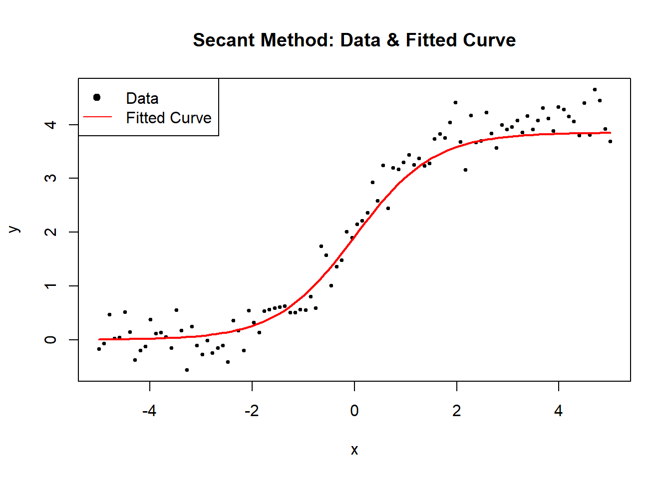
Figure 6.7: Secant Method
6.2.2.2 Grid Search
Grid Search (GS) is a brute-force optimization method that systematically explores a grid of possible parameter values to identify the combination that minimizes the residual sum of squares (RSS). Unlike gradient-based optimization, which moves iteratively towards a minimum, grid search evaluates all predefined parameter combinations, making it robust but computationally expensive.
Grid search is particularly useful when:
The function is highly nonlinear, making gradient methods unreliable.
The parameter space is small, allowing exhaustive search.
A global minimum is needed, and prior knowledge about parameter ranges exists.
The goal of Grid Search is to find an optimal parameter set \(\hat{\theta}\) that minimizes the Sum of Squared Errors (SSE):
\[ \hat{\theta} = \arg\min_{\theta \in \Theta} SSE(\theta), \]
where:
\[ SSE(\theta) = \sum_{i=1}^{n} (y_i - f(x_i; \theta))^2. \]
Grid search discretizes the search space \(\Theta\) into a finite set of candidate values for each parameter:
\[ \Theta = \theta_1 \times \theta_2 \times \dots \times \theta_p. \]
The accuracy of the solution depends on the grid resolution—a finer grid leads to better accuracy but higher computational cost.
Grid Search Algorithm
- Define a grid of possible values for each parameter.
- Evaluate SSE for each combination of parameters.
- Select the parameter set that minimizes SSE.
# Define a numerically stable logistic function
safe_exp <- function(x) {
    return(ifelse(x > 700, Inf, exp(pmin(x, 700))))  # Prevent overflow
}

# Define the logistic growth model
nonlinear_model <- function(theta, x) {
    return(theta[1] / (1 + safe_exp(-theta[2] * (x - theta[3]))))
}

# Define the Sum of Squared Errors (SSE) function
sse <- function(theta, x, y) {
    predictions <- nonlinear_model(theta, x)
    return(sum((y - predictions)^2))
}

# Grid Search Optimization
grid_search_optimization <- function(x, y, grid_size = 10) {
    # Define grid of parameter values
    A_values <- seq(2, 6, length.out = grid_size)
    B_values <- seq(0.5, 3, length.out = grid_size)
    C_values <- seq(-2, 2, length.out = grid_size)

    # Generate all combinations of parameters
    param_grid <- expand.grid(A = A_values, B = B_values, C = C_values)

    # Evaluate SSE for each parameter combination
    param_grid$SSE <- apply(param_grid, 1, function(theta) {
        sse(as.numeric(theta[1:3]), x, y)
    })

    # Select the best parameter set
    best_params <- param_grid[which.min(param_grid$SSE), 1:3]
    return(as.numeric(best_params))
}

# Generate synthetic data
set.seed(123)
x <- seq(-5, 5, length.out = 100)
true_theta <- c(4, 1.5, 0)  # True parameters (A, B, C)
y <- nonlinear_model(true_theta, x) + rnorm(length(x), sd = 0.3)

# Run Grid Search
estimated_theta <- grid_search_optimization(x, y, grid_size = 20)

# Display results
cat("Estimated parameters (A, B, C) using Grid Search:\n")
#> Estimated parameters (A, B, C) using Grid Search:
print(estimated_theta)
#> [1] 4.1052632 1.4210526 0.1052632
# Plot data and fitted curve
plot(
x, y,
main = "Grid Search: Nonlinear Regression Optimization",
pch = 19,
cex = 0.5,
xlab = "x",
ylab = "y"
)
curve(
nonlinear_model(estimated_theta, x),
from = min(x),
to = max(x),
add = TRUE,
col = "red",
lwd = 2
)
legend(
"topleft",
legend = c("Data", "Fitted Curve"),
pch = c(19, NA),
lty = c(NA, 1),
col = c("black", "red")
)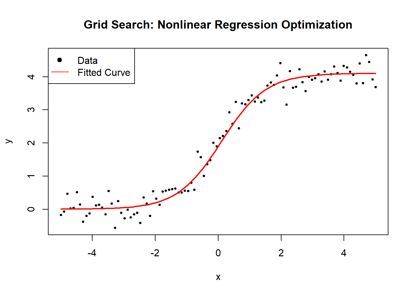
Figure 6.8: Grid Search: Nonlinear Regression Optimization
6.2.2.3 Nelder-Mead (Simplex)
The Nelder-Mead algorithm, also known as the Simplex method, is a derivative-free optimization algorithm that iteratively adjusts a geometric shape (simplex) to find the minimum of an objective function. It is particularly useful for nonlinear regression when gradient-based methods fail due to non-differentiability or noisy function evaluations.
Nelder-Mead is particularly useful when:
The function is non-differentiable or noisy.
Gradient-based methods are unreliable.
The parameter space is low-dimensional.
The goal of Nelder-Mead is to find an optimal parameter set \(\hat{\theta}\) that minimizes the Sum of Squared Errors (SSE):
\[ \hat{\theta} = \arg\min_{\theta} SSE(\theta), \]
where:
\[ SSE(\theta) = \sum_{i=1}^{n} (y_i - f(x_i; \theta))^2. \]
1. Simplex Representation
The algorithm maintains a simplex, a geometric shape with \(p+1\) vertices for a \(p\)-dimensional parameter space.
Each vertex represents a parameter vector:
\[ S = \{ \theta_1, \theta_2, \dots, \theta_{p+1} \}. \]
2. Simplex Operations
At each iteration, the algorithm updates the simplex based on the objective function values at each vertex:
Reflection: Reflect the worst point \(\theta_h\) across the centroid.
\[ \theta_r = \theta_c + \alpha (\theta_c - \theta_h) \]
Expansion: If reflection improves the objective, expand the step.
\[ \theta_e = \theta_c + \gamma (\theta_r - \theta_c) \]
Contraction: If reflection worsens the objective, contract towards the centroid.
\[ \theta_c = \theta_c + \rho (\theta_h - \theta_c) \]
Shrink: If contraction fails, shrink the simplex.
\[ \theta_i = \theta_1 + \sigma (\theta_i - \theta_1), \quad \forall i > 1 \]
where:
\(\alpha = 1\) (reflection coefficient),
\(\gamma = 2\) (expansion coefficient),
\(\rho = 0.5\) (contraction coefficient),
\(\sigma = 0.5\) (shrink coefficient).
The process continues until convergence.
Nelder-Mead Algorithm
- Initialize a simplex with \(p+1\) vertices.
- Evaluate SSE at each vertex.
- Perform reflection, expansion, contraction, or shrink operations.
- Repeat until convergence.
# Load required library
library(stats)


# Define a numerically stable logistic function
safe_exp <- function(x) {
    return(ifelse(x > 700, Inf, exp(pmin(x, 700))))  # Prevent overflow
}

# Define the logistic growth model
nonlinear_model <- function(theta, x) {
    return(theta[1] / (1 + safe_exp(-theta[2] * (x - theta[3]))))
}

# Define the Sum of Squared Errors (SSE) function
sse <- function(theta, x, y) {
    predictions <- nonlinear_model(theta, x)
    return(sum((y - predictions) ^ 2))
}

# Nelder-Mead Optimization
nelder_mead_optimization <- function(x, y) {
    # Initial guess for parameters
    initial_guess <- c(2, 1, 0)

    # Run Nelder-Mead optimization
    result <- optim(
        par = initial_guess,
        fn = sse,
        x = x,
        y = y,
        method = "Nelder-Mead",
        control = list(maxit = 500)
    )

    return(result$par)  # Return optimized parameters
}

# Generate synthetic data
set.seed(123)
x <- seq(-5, 5, length.out = 100)
true_theta <- c(4, 1.5, 0)  # True parameters (A, B, C)
y <- nonlinear_model(true_theta, x) + rnorm(length(x), sd = 0.3)

# Run Nelder-Mead Optimization
estimated_theta <- nelder_mead_optimization(x, y)

# Display results
cat("Estimated parameters (A, B, C) using Nelder-Mead:\n")
#> Estimated parameters (A, B, C) using Nelder-Mead:
print(estimated_theta)
#> [1] 4.06873116 1.42759898 0.01119379
# Plot data and fitted curve
plot(
x,
y,
main = "Nelder-Mead: Nonlinear Regression Optimization",
pch = 19,
cex = 0.5,
xlab = "x",
ylab = "y"
)
curve(
nonlinear_model(estimated_theta, x),
from = min(x),
to = max(x),
add = TRUE,
col = "red",
lwd = 2
)
legend(
"topleft",
legend = c("Data", "Fitted Curve"),
pch = c(19, NA),
lty = c(NA, 1),
col = c("black", "red")
)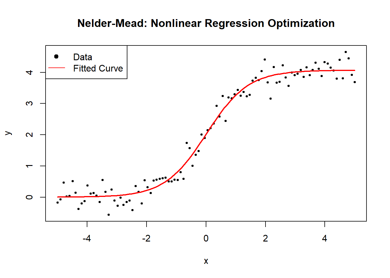
Figure 6.9: Nelder–Mead: Nonlinear Regression Optimization
6.2.2.4 Powell’s Method
Powell’s Method is a derivative-free optimization algorithm that minimizes a function without using gradients. It works by iteratively refining a set of search directions to efficiently navigate the parameter space. Unlike Nelder-Mead (Simplex), which adapts a simplex, Powell’s method builds an orthogonal basis of search directions.
Powell’s method is particularly useful when:
The function is non-differentiable or noisy.
Gradient-based methods are unreliable.
The parameter space is low-to-moderate dimensional.
The goal of Powell’s Method is to find an optimal parameter set \(\hat{\theta}\) that minimizes the Sum of Squared Errors (SSE):
\[ \hat{\theta} = \arg\min_{\theta} SSE(\theta), \]
where:
\[ SSE(\theta) = \sum_{i=1}^{n} (y_i - f(x_i; \theta))^2. \]
1. Search Directions
Powell’s method maintains a set of search directions \(\mathbf{d}_1, \mathbf{d}_2, \dots, \mathbf{d}_p\):
\[ D = \{ \mathbf{d}_1, \mathbf{d}_2, ..., \mathbf{d}_p \}. \]
Initially, these directions are chosen as unit basis vectors (each optimizing a single parameter independently).
2. Line Minimization
For each direction \(\mathbf{d}_j\), Powell’s method performs a 1D optimization:
\[ \theta' = \theta + \lambda \mathbf{d}_j, \]
where \(\lambda\) is chosen to minimize \(SSE(\theta')\).
3. Updating Search Directions
After optimizing along all directions:
- The largest improvement direction \(\mathbf{d}_{\max}\) is replaced with:
\[ \mathbf{d}_{\text{new}} = \theta_{\text{final}} - \theta_{\text{initial}}. \]
- The new direction set is orthogonalized using Gram-Schmidt.
This ensures efficient exploration of the parameter space.
4. Convergence Criteria
Powell’s method stops when function improvement is below a tolerance level:
\[ |SSE(\theta_{t+1}) - SSE(\theta_t)| < \epsilon. \]
Powell’s Method Algorithm
- Initialize search directions (standard basis vectors).
- Perform 1D line searches along each direction.
- Update the search directions based on the largest improvement.
- Repeat until convergence.
# Load required library
library(stats)

# Define a numerically stable logistic function
safe_exp <- function(x) {
    return(ifelse(x > 700, Inf, exp(pmin(x, 700))))  # Prevent overflow
}

# Define the logistic growth model
nonlinear_model <- function(theta, x) {
    return(theta[1] / (1 + safe_exp(-theta[2] * (x - theta[3]))))
}

# Define the Sum of Squared Errors (SSE) function
sse <- function(theta, x, y) {
    predictions <- nonlinear_model(theta, x)
    return(sum((y - predictions) ^ 2))
}

# Powell's Method Optimization
powell_optimization <- function(x, y) {
    # Initial guess for parameters
    initial_guess <- c(2, 1, 0)

    # Run Powell’s optimization (via BFGS without gradient)
    result <- optim(
        par = initial_guess,
        fn = sse,
        x = x,
        y = y,
        method = "BFGS",
        control = list(maxit = 500),
        gr = NULL  # No gradient used
    )

    return(result$par)  # Return optimized parameters
}

# Generate synthetic data
set.seed(123)
x <- seq(-5, 5, length.out = 100)
true_theta <- c(4, 1.5, 0)  # True parameters (A, B, C)
y <- nonlinear_model(true_theta, x) + rnorm(length(x), sd = 0.3)

# Run Powell's Method Optimization
estimated_theta <- powell_optimization(x, y)

# Display results
cat("Estimated parameters (A, B, C) using Powell’s Method:\n")
#> Estimated parameters (A, B, C) using Powell’s Method:
print(estimated_theta)
#> [1] 4.06876538 1.42765687 0.01128753
# Plot data and fitted curve
plot(
x,
y,
main = "Powell's Method: Nonlinear Regression Optimization",
pch = 19,
cex = 0.5,
xlab = "x",
ylab = "y"
)
curve(
nonlinear_model(estimated_theta, x),
from = min(x),
to = max(x),
add = TRUE,
col = "red",
lwd = 2
)
legend(
"topleft",
legend = c("Data", "Fitted Curve"),
pch = c(19, NA),
lty = c(NA, 1),
col = c("black", "red")
)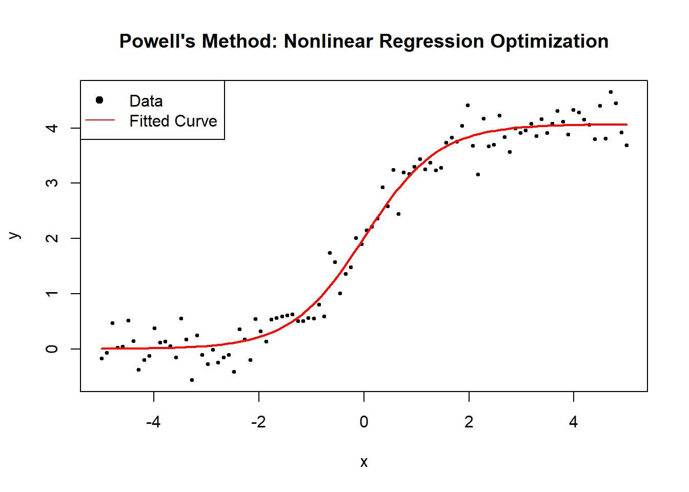
Figure 6.10: Powell’s Method: Nonlinear Regression Optimization
6.2.2.5 Random Search
Random Search (RS) is a simple yet effective optimization algorithm that explores the search space by randomly sampling candidate solutions. Unlike grid search, which evaluates all predefined parameter combinations, random search selects a random subset, reducing computational cost.
Random search is particularly useful when:
The search space is large, making grid search impractical.
Gradient-based methods fail due to non-differentiability or noisy data.
The optimal region is unknown, making global exploration essential.
The goal of Random Search is to find an optimal parameter set \(\hat{\theta}\) that minimizes the Sum of Squared Errors (SSE):
\[ \hat{\theta} = \arg\min_{\theta \in \Theta} SSE(\theta), \]
where:
\[ SSE(\theta) = \sum_{i=1}^{n} (y_i - f(x_i; \theta))^2. \]
Unlike grid search, random search does not evaluate all parameter combinations but instead randomly samples a subset:
\[ \Theta_{\text{sampled}} \subset \Theta. \]
The accuracy of the solution depends on the number of random samples—a higher number increases the likelihood of finding a good solution.
Random Search Algorithm
- Define a random sampling range for each parameter.
- Randomly sample \(N\) parameter sets.
- Evaluate SSE for each sampled set.
- Select the parameter set that minimizes SSE.
# Load required library
library(stats)

# Define a numerically stable logistic function
safe_exp <- function(x) {
  return(ifelse(x > 700, Inf, exp(pmin(x, 700))))  # Prevent overflow
}

# Define the logistic growth model
nonlinear_model <- function(theta, x) {
  return(theta[1] / (1 + safe_exp(-theta[2] * (x - theta[3]))))
}

# Define the Sum of Squared Errors (SSE) function
sse <- function(theta, x, y) {
  predictions <- nonlinear_model(theta, x)
  return(sum((y - predictions) ^ 2))
}

# Random Search Optimization
random_search_optimization <- function(x, y, num_samples = 100) {
  # Define parameter ranges
  A_range <-
    runif(num_samples, 2, 6)   # Random values between 2 and 6
  B_range <-
    runif(num_samples, 0.5, 3) # Random values between 0.5 and 3
  C_range <-
    runif(num_samples,-2, 2)  # Random values between -2 and 2

  # Initialize best parameters
  best_theta <- NULL
  best_sse <- Inf

  # Evaluate randomly sampled parameter sets
  for (i in 1:num_samples) {
    theta <- c(A_range[i], B_range[i], C_range[i])
    current_sse <- sse(theta, x, y)

    if (current_sse < best_sse) {
      best_sse <- current_sse
      best_theta <- theta
    }
  }

  return(best_theta)
}

# Generate synthetic data
set.seed(123)
x <- seq(-5, 5, length.out = 100)
true_theta <- c(4, 1.5, 0)  # True parameters (A, B, C)
y <- nonlinear_model(true_theta, x) + rnorm(length(x), sd = 0.3)

# Run Random Search
estimated_theta <-
  random_search_optimization(x, y, num_samples = 500)

# Display results
cat("Estimated parameters (A, B, C) using Random Search:\n")
#> Estimated parameters (A, B, C) using Random Search:
print(estimated_theta)
#> [1] 4.0893431 1.4687456 0.1024474
# Plot data and fitted curve
plot(
x,
y,
main = "Random Search: Nonlinear Regression Optimization",
pch = 19,
cex = 0.5,
xlab = "x",
ylab = "y"
)
curve(
nonlinear_model(estimated_theta, x),
from = min(x),
to = max(x),
add = TRUE,
col = "red",
lwd = 2
)
legend(
"topleft",
legend = c("Data", "Fitted Curve"),
pch = c(19, NA),
lty = c(NA, 1),
col = c("black", "red")
)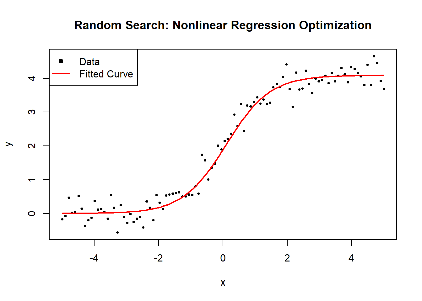
Figure 6.11: Random Search: Nonlinear Regression Optimization
6.2.2.6 Hooke-Jeeves Pattern Search
Hooke-Jeeves Pattern Search is a derivative-free optimization algorithm that searches for an optimal solution by exploring and adjusting parameter values iteratively. Unlike gradient-based methods, it does not require differentiability, making it effective for non-smooth and noisy functions.
Hooke-Jeeves is particularly useful when:
The function is non-differentiable or noisy.
Gradient-based methods are unreliable.
The parameter space is low-to-moderate dimensional.
The goal of Hooke-Jeeves Pattern Search is to find an optimal parameter set \(\hat{\theta}\) that minimizes the Sum of Squared Errors (SSE):
\[ \hat{\theta} = \arg\min_{\theta} SSE(\theta), \]
where:
\[ SSE(\theta) = \sum_{i=1}^{n} (y_i - f(x_i; \theta))^2. \]
1. Exploratory Moves
At each iteration, the algorithm perturbs each parameter to find a lower SSE:
\[ \theta' = \theta \pm \delta. \]
If a new parameter \(\theta'\) reduces SSE, it becomes the new base point.
2. Pattern Moves
After an improvement, the algorithm accelerates movement in the promising direction:
\[ \theta_{\text{new}} = \theta_{\text{old}} + (\theta_{\text{old}} - \theta_{\text{prev}}). \]
This speeds up convergence towards an optimum.
3. Step Size Adaptation
If no improvement is found, the step size \(\delta\) is reduced:
\[ \delta_{\text{new}} = \beta \cdot \delta. \]
where \(\beta < 1\) is a reduction factor.
4. Convergence Criteria
The algorithm stops when step size is sufficiently small:
\[ \delta < \epsilon. \]
Hooke-Jeeves Algorithm
- Initialize a starting point \(\theta\) and step size \(\delta\).
- Perform exploratory moves in each parameter direction.
- If improvement is found, perform pattern moves.
- Reduce step size if no improvement is found.
- Repeat until convergence.
# Load required library
library(stats)

# Define a numerically stable logistic function
safe_exp <- function(x) {
    return(ifelse(x > 700, Inf, exp(pmin(x, 700))))  # Prevent overflow
}

# Define the logistic growth model
nonlinear_model <- function(theta, x) {
    return(theta[1] / (1 + safe_exp(-theta[2] * (x - theta[3]))))
}

# Define the Sum of Squared Errors (SSE) function
sse <- function(theta, x, y) {
    predictions <- nonlinear_model(theta, x)
    return(sum((y - predictions) ^ 2))
}

# Hooke-Jeeves Pattern Search Optimization
hooke_jeeves_optimization <-
    function(x,
             y,
             step_size = 0.5,
             tol = 1e-6,
             max_iter = 500) {
        # Initial guess for parameters
        theta <- c(2, 1, 0)
        best_sse <- sse(theta, x, y)
        step <- step_size
        iter <- 0

        while (step > tol & iter < max_iter) {
            iter <- iter + 1
            improved <- FALSE
            new_theta <- theta

            # Exploratory move in each parameter direction
            for (i in 1:length(theta)) {
                for (delta in c(step,-step)) {
                    theta_test <- new_theta
                    theta_test[i] <- theta_test[i] + delta
                    sse_test <- sse(theta_test, x, y)

                    if (sse_test < best_sse) {
                        best_sse <- sse_test
                        new_theta <- theta_test
                        improved <- TRUE
                    }
                }
            }

            # Pattern move if improvement found
            if (improved) {
                theta <- 2 * new_theta - theta
                best_sse <- sse(theta, x, y)
            } else {
                step <- step / 2  # Reduce step size
            }
        }

        return(theta)
    }

# Generate synthetic data
set.seed(123)
x <- seq(-5, 5, length.out = 100)
true_theta <- c(4, 1.5, 0)  # True parameters (A, B, C)
y <- nonlinear_model(true_theta, x) + rnorm(length(x), sd = 0.3)

# Run Hooke-Jeeves Optimization
estimated_theta <- hooke_jeeves_optimization(x, y)

# Display results
cat("Estimated parameters (A, B, C) using Hooke-Jeeves:\n")
#> Estimated parameters (A, B, C) using Hooke-Jeeves:
print(estimated_theta)
#> [1] 4 1 0
# Plot data and fitted curve
plot(
x,
y,
main = "Hooke-Jeeves: Nonlinear Regression Optimization",
pch = 19,
cex = 0.5,
xlab = "x",
ylab = "y"
)
curve(
nonlinear_model(estimated_theta, x),
from = min(x),
to = max(x),
add = TRUE,
col = "red",
lwd = 2
)
legend(
"topleft",
legend = c("Data", "Fitted Curve"),
pch = c(19, NA),
lty = c(NA, 1),
col = c("black", "red")
)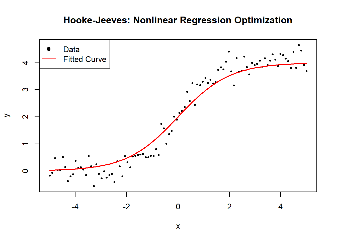
Figure 6.12: Hooke–Jeeves: Nonlinear Regression Optimization
6.2.2.7 Bisection Method
The Bisection Method is a fundamental numerical technique primarily used for root finding, but it can also be adapted for optimization problems where the goal is to minimize or maximize a nonlinear function.
In nonlinear regression, optimization often involves finding the parameter values that minimize the sum of squared errors (SSE):
\[ \hat{\theta} = \arg\min_{\theta} SSE(\theta) \]
where:
\[ SSE(\theta) = \sum_{i=1}^{n} \left( y_i - f(x_i; \theta) \right)^2. \]
Since the minimum of a function occurs where the derivative equals zero, we apply the Bisection Method to the derivative of the SSE function:
\[ \frac{d}{d\theta} SSE(\theta) = 0. \]
This transforms the optimization problem into a root-finding problem.
The Bisection Method is based on the Intermediate Value Theorem, which states:
If a continuous function \(f(\theta)\) satisfies \(f(\theta_a) \cdot f(\theta_b) < 0\),
then there exists at least one root in the interval \((\theta_a, \theta_b)\).
For optimization, we apply this principle to the first derivative of the objective function \(Q(\theta)\):
\[ Q'(\theta) = 0. \]
Step-by-Step Algorithm for Optimization
- Choose an interval \([\theta_a, \theta_b]\) such that: \[ Q'(\theta_a) \cdot Q'(\theta_b) < 0. \]
- Compute the midpoint: \[ \theta_m = \frac{\theta_a + \theta_b}{2}. \]
- Evaluate \(Q'(\theta_m)\):
- If \(Q'(\theta_m) = 0\), then \(\theta_m\) is the optimal point.
- If \(Q'(\theta_a) \cdot Q'(\theta_m) < 0\), set \(\theta_b = \theta_m\).
- Otherwise, set \(\theta_a = \theta_m\).
- Repeat until convergence: \[ |\theta_b - \theta_a| < \epsilon. \]
Determining the Nature of the Critical Point
Since the Bisection Method finds a stationary point, we use the second derivative test to classify it:
- If \(Q''(\theta) > 0\), the point is a local minimum.
- If \(Q''(\theta) < 0\), the point is a local maximum.
For nonlinear regression, we expect \(Q(\theta) = SSE(\theta)\), so the solution found by Bisection should be a minimum.
# Load required library
library(stats)

# Define a numerically stable logistic function
safe_exp <- function(x) {
    return(ifelse(x > 700, Inf, exp(pmin(x, 700))))  # Prevent overflow
}

# Define the logistic growth model
nonlinear_model <- function(theta, x) {
    return(theta[1] / (1 + safe_exp(-theta[2] * (x - theta[3]))))
}

# Define the Sum of Squared Errors (SSE) function for optimization
sse <- function(theta, x, y) {
    predictions <- nonlinear_model(theta, x)
    return(sum((y - predictions)^2))
}

# Optimize all three parameters simultaneously
find_optimal_parameters <- function(x, y) {
    # Initial guess for parameters (based on data)
    initial_guess <- c(max(y), 1, median(x))

    # Bounds for parameters
    lower_bounds <- c(0.1, 0.01, min(x))  # Ensure positive scaling
    upper_bounds <- c(max(y) * 2, 10, max(x))

    # Run optim() with L-BFGS-B (bounded optimization)
    result <- optim(
        par = initial_guess,
        fn = sse,
        x = x, y = y,
        method = "L-BFGS-B",
        lower = lower_bounds,
        upper = upper_bounds
    )

    return(result$par)  # Extract optimized parameters
}

# Generate synthetic data
set.seed(123)
x <- seq(-5, 5, length.out = 100)
true_theta <- c(4, 1.5, 0)  # True parameters (A, B, C)
y <- nonlinear_model(true_theta, x) + rnorm(length(x), sd = 0.3)

# Find optimal parameters using optim()
estimated_theta <- find_optimal_parameters(x, y)

# Display results
cat("Estimated parameters (A, B, C) using optim():\n")
#> Estimated parameters (A, B, C) using optim():
print(estimated_theta)
#> [1] 4.06876536 1.42765688 0.01128756
# Plot data and fitted curve
plot(
x, y,
main = "Optim(): Nonlinear Regression Optimization",
pch = 19,
cex = 0.5,
xlab = "x",
ylab = "y"
)
curve(
nonlinear_model(estimated_theta, x),
from = min(x),
to = max(x),
add = TRUE,
col = "red",
lwd = 2
)
legend(
"topleft",
legend = c("Data", "Fitted Curve"),
pch = c(19, NA),
lty = c(NA, 1),
col = c("black", "red")
)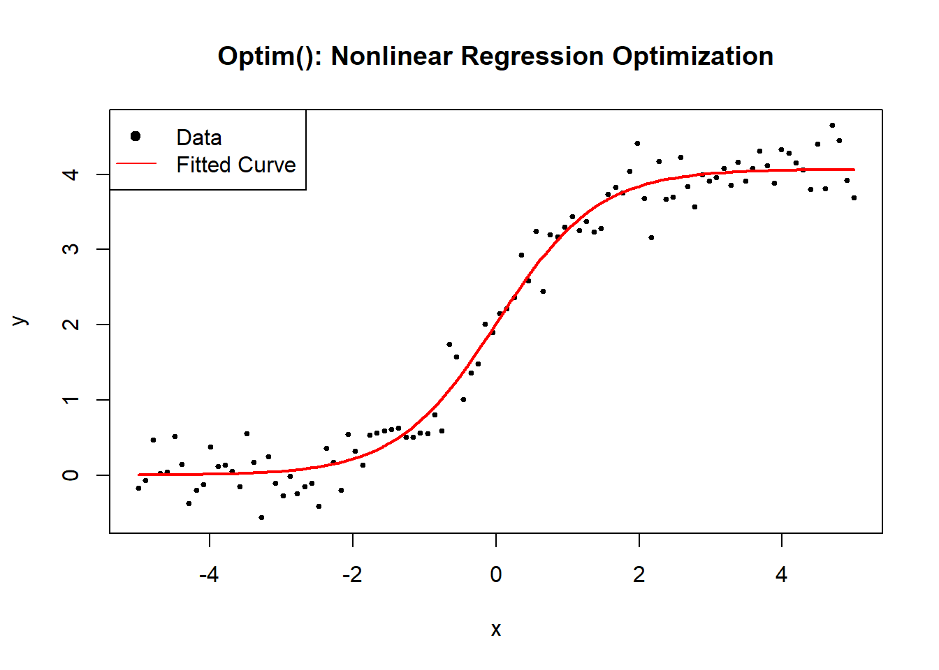
Figure 6.13: Optim(): Nonlinear Regression Optimization
6.2.3 Stochastic Heuristic
6.2.3.1 Differential Evolution Algorithm
The Differential Evolution (DE) Algorithm is a stochastic, population-based optimization algorithm that is widely used for solving complex global optimization problems. Unlike gradient-based methods such as Newton’s method or the Secant method, DE does not require derivatives and is well-suited for optimizing non-differentiable, nonlinear, and multimodal functions.
Key Features of Differential Evolution
- Population-based approach: Maintains a population of candidate solutions instead of a single point.
- Mutation and crossover: Introduces variations to explore the search space.
- Selection mechanism: Retains the best candidates for the next generation.
- Global optimization: Avoids local minima by using stochastic search strategies.
Mathematical Formulation of Differential Evolution
Differential Evolution operates on a population of candidate solutions \(\{\theta_i\}\), where each \(\theta_i\) is a vector of parameters. The algorithm iteratively updates the population using three main operations:
1. Mutation
For each candidate solution \(\theta_i\), a mutant vector \(\mathbf{v}_i^{(j)}\) is generated as:
\[ \mathbf{v}_i^{(j)} = \mathbf{\theta}_{r_1}^{(j)} + F \cdot (\mathbf{\theta}_{r_2}^{(j)} - \mathbf{\theta}_{r_3}^{(j)}) \]
where:
\(\mathbf{\theta}_{r_1}, \mathbf{\theta}_{r_2}, \mathbf{\theta}_{r_3}\) are randomly selected distinct vectors from the population.
\(F \in (0,2)\) is the mutation factor controlling the step size.
2. Crossover
A trial vector \(\mathbf{u}_i^{(j)}\) is generated by combining the mutant vector \(\mathbf{v}_i^{(j)}\) with the original solution \(\mathbf{\theta}_i^{(j)}\):
\[ u_{i,k}^{(j)} = \begin{cases} v_{i,k}^{(j)} & \text{if } rand_k \leq C_r \text{ or } k = k_{\text{rand}}, \\ \theta_{i,k}^{(j)} & \text{otherwise}. \end{cases} \]
where:
\(C_r \in (0,1)\) is the crossover probability.
\(rand_k\) is a random value between 0 and 1.
\(k_{\text{rand}}\) ensures at least one parameter is mutated.
3. Selection
The new candidate solution is accepted only if it improves the objective function:
\[ \mathbf{\theta}_i^{(j+1)} = \begin{cases} \mathbf{u}_i^{(j)} & \text{if } Q(\mathbf{u}_i^{(j)}) < Q(\mathbf{\theta}_i^{(j)}), \\ \mathbf{\theta}_i^{(j)} & \text{otherwise}. \end{cases} \]
where \(Q(\theta)\) is the objective function (e.g., sum of squared errors in regression problems).
Algorithm: Differential Evolution for Nonlinear Optimization
- Initialize a population of candidate solutions.
- Evaluate the objective function for each candidate.
- Mutate individuals using a difference strategy.
- Apply crossover to create trial solutions.
- Select individuals based on their fitness (objective function value).
- Repeat until convergence (or a stopping criterion is met).
# Load required library
library(DEoptim)

# Define a nonlinear function (logistic model)
nonlinear_model <- function(theta, x) {
    return(theta[1] / (1 + exp(-theta[2] * (x - theta[3]))))
}

# Define the Sum of Squared Errors (SSE) function
sse <- function(theta, x, y) {
    return(sum((y - nonlinear_model(theta, x))^2))
}

# Generate synthetic data
set.seed(123)
x <- seq(-5, 5, length.out = 100)
true_theta <- c(4, 1.5, 0)  # True parameters (A, B, C)
y <- nonlinear_model(true_theta, x) + rnorm(length(x), sd = 0.3)

# Define the objective function for DEoptim
objective_function <- function(theta) {
    return(sse(theta, x, y))
}

# Define parameter bounds
lower_bounds <- c(0, 0, -5)
upper_bounds <- c(10, 5, 5)

# Run Differential Evolution Algorithm
de_result <-
    DEoptim(
        objective_function,
        lower_bounds,
        upper_bounds,
        DEoptim.control(
            NP = 50,
            itermax = 100,
            F = 0.8,
            CR = 0.9,
            trace = F
        )
    )

# Extract optimized parameters
estimated_theta <- de_result$optim$bestmem

# Display estimated parameters
cat("Estimated parameters (A, B, C) using Differential Evolution:\n")
#> Estimated parameters (A, B, C) using Differential Evolution:
print(estimated_theta)
#>       par1       par2       par3
#> 4.06876562 1.42765614 0.01128768
# Plot data and fitted curve
plot(
x,
y,
main = "Differential Evolution: Data & Fitted Curve",
pch = 19,
cex = 0.5,
xlab = "x",
ylab = "y"
)
curve(
nonlinear_model(estimated_theta, x),
from = -5,
to = 5,
add = TRUE,
col = "red",
lwd = 2
)
legend(
"topleft",
legend = c("Data", "Fitted Curve"),
pch = c(19, NA),
lty = c(NA, 1),
col = c("black", "red")
)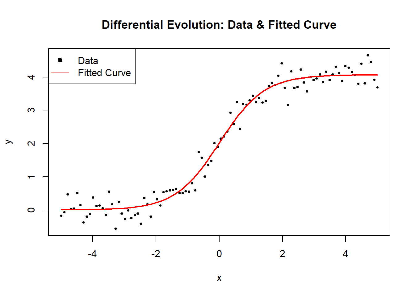
Figure 6.14: Differential Evolution
6.2.3.2 Simulated Annealing
Simulated Annealing (SA) is a probabilistic global optimization algorithm inspired by annealing in metallurgy, where a material is heated and slowly cooled to remove defects. In optimization, SA gradually refines a solution by exploring the search space, allowing occasional jumps to escape local minima, before converging to an optimal solution.
Simulated Annealing is particularly useful when:
The function is highly nonlinear and multimodal.
Gradient-based methods struggle due to non-differentiability or poor initialization.
A global minimum is needed, rather than a local one.
1. Energy Function (Objective Function)
The goal of SA is to minimize an objective function \(Q(\theta)\). For nonlinear regression, this is the Sum of Squared Errors (SSE):
\[ Q(\theta) = SSE(\theta) = \sum_{i=1}^{n} (y_i - f(x_i; \theta))^2. \]
2. Probability of Acceptance
At each step, SA randomly perturbs the parameters \(\theta\) to create a new candidate solution \(\theta'\) and evaluates the change in SSE:
\[ \Delta Q = Q(\theta') - Q(\theta). \]
The Metropolis Criterion determines whether to accept the new solution:
\[ P(\text{accept}) = \begin{cases} 1, & \text{if } \Delta Q < 0 \quad \text{(new solution improves fit)} \\ \exp\left( -\frac{\Delta Q}{T} \right), & \text{if } \Delta Q \geq 0 \quad \text{(accept with probability)}. \end{cases} \]
where:
\(T\) is the temperature that gradually decreases over iterations.
Worse solutions are accepted with small probability to escape local minima.
3. Cooling Schedule
The temperature follows a cooling schedule:
\[ T_k = \alpha T_{k-1}, \]
where \(\alpha \in (0,1)\) is a decay factor that controls cooling speed.
Simulated Annealing Algorithm
- Initialize parameters \(\theta\) randomly.
- Set an initial temperature \(T_0\) and cooling rate \(\alpha\).
- Repeat for max iterations:
- Generate perturbed candidate \(\theta'\).
- Compute \(\Delta Q = Q(\theta') - Q(\theta)\).
- Accept if \(\Delta Q < 0\) or with probability \(\exp(-\Delta Q / T)\).
- Reduce temperature: \(T \leftarrow \alpha T\).
- Return the best solution found.
# Load required library
library(stats)

# Define a numerically stable logistic function
safe_exp <- function(x) {
    return(ifelse(x > 700, Inf, exp(pmin(x, 700))))  # Prevent overflow
}

# Define the logistic growth model
nonlinear_model <- function(theta, x) {
    return(theta[1] / (1 + safe_exp(-theta[2] * (x - theta[3]))))
}

# Define the Sum of Squared Errors (SSE) function
sse <- function(theta, x, y) {
    predictions <- nonlinear_model(theta, x)
    return(sum((y - predictions) ^ 2))
}

# Simulated Annealing Algorithm
simulated_annealing <-
    function(x,
             y,
             initial_theta,
             T_init = 1.0,
             alpha = 0.99,
             max_iter = 5000) {
        # Initialize parameters
        theta <- initial_theta
        best_theta <- theta
        best_sse <- sse(theta, x, y)
        T <- T_init  # Initial temperature

        for (iter in 1:max_iter) {
            # Generate new candidate solution (small random perturbation)
            theta_new <- theta + rnorm(length(theta), mean = 0, sd = T)

            # Compute new SSE
            sse_new <- sse(theta_new, x, y)

            # Compute change in SSE
            delta_Q <- sse_new - best_sse

            # Acceptance criteria
            if (delta_Q < 0 || runif(1) < exp(-delta_Q / T)) {
                theta <- theta_new
                best_sse <- sse_new
                best_theta <- theta_new
            }

            # Reduce temperature
            T <- alpha * T

            # Stopping condition (very low temperature)
            if (T < 1e-6)
                break
        }

        return(best_theta)
    }

# Generate synthetic data
set.seed(123)
x <- seq(-5, 5, length.out = 100)
true_theta <- c(4, 1.5, 0)  # True parameters (A, B, C)
y <- nonlinear_model(true_theta, x) + rnorm(length(x), sd = 0.3)

# Initial guess
initial_theta <-
    c(runif(1, 1, 5), runif(1, 0.1, 3), runif(1,-2, 2))

# Run Simulated Annealing
estimated_theta <- simulated_annealing(x, y, initial_theta)

# Display results
cat("Estimated parameters (A, B, C) using Simulated Annealing:\n")
#> Estimated parameters (A, B, C) using Simulated Annealing:
print(estimated_theta)
#> [1] 4.07180419 1.41457906 0.01422147
# Plot data and fitted curve
plot(
x,
y,
main = "Simulated Annealing: Nonlinear Regression Optimization",
pch = 19,
cex = 0.5,
xlab = "x",
ylab = "y"
)
curve(
nonlinear_model(estimated_theta, x),
from = min(x),
to = max(x),
add = TRUE,
col = "red",
lwd = 2
)
legend(
"topleft",
legend = c("Data", "Fitted Curve"),
pch = c(19, NA),
lty = c(NA, 1),
col = c("black", "red")
)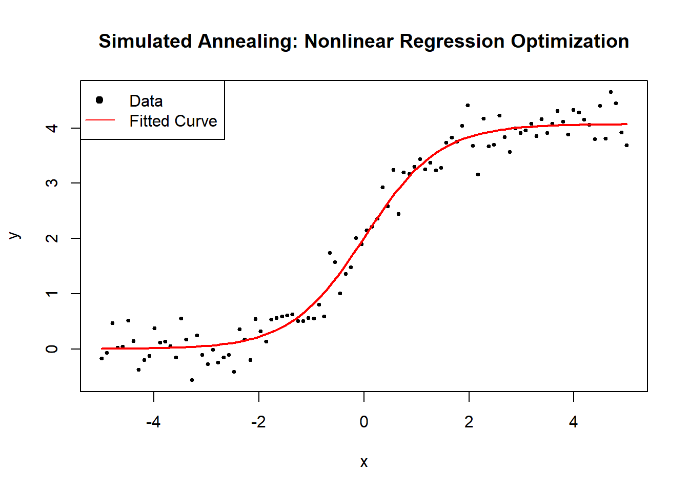
Figure 6.15: Simulated Annealing: Nonlinear Regression Optimization
6.2.3.3 Genetic Algorithm
Genetic Algorithms (GA) are a class of evolutionary algorithms inspired by the principles of natural selection and genetics. Unlike deterministic optimization techniques, GA evolves a population of candidate solutions over multiple generations, using genetic operators such as selection, crossover, and mutation.
GA is particularly useful when:
The function is nonlinear, non-differentiable, or highly multimodal.
Gradient-based methods fail due to rugged function landscapes.
A global minimum is required, rather than a local one.
The goal of a Genetic Algorithm is to find an optimal solution $\hat{\theta}$ that minimizes an objective function:
\[ \hat{\theta} = \arg\min_{\theta} SSE(\theta), \]
where:
\[ SSE(\theta) = \sum_{i=1}^{n} (y_i - f(x_i; \theta))^2. \]
1. Population Representation
Each candidate solution (individual) is represented as a chromosome, which is simply a vector of parameters: \[ \theta = (\theta_1, \theta_2, \theta_3) \]
An entire population consists of multiple such solutions.
2. Selection
Each individual’s fitness is evaluated using:
\[ \text{Fitness}(\theta) = -SSE(\theta) \]
We use Tournament Selection or Roulette Wheel Selection to choose parents for reproduction.
3. Crossover (Recombination)
A new solution \(\theta'\) is generated by combining two parents:
\[\theta' = \alpha \theta_{\text{parent1}} + (1 - \alpha) \theta_{\text{parent2}}, \quad \alpha \sim U(0,1).\]
4. Mutation
Random small changes are introduced to increase diversity:
\[\theta_i' = \theta_i + \mathcal{N}(0, \sigma),\]
where \(\mathcal{N}(0, \sigma)\) is a small Gaussian perturbation.
5. Evolutionary Cycle
The algorithm iterates through:
Selection
Crossover
Mutation
Survival of the fittest
Termination when convergence is reached.
# Load required library
library(GA)

# Define a numerically stable logistic function
safe_exp <- function(x) {
    return(ifelse(x > 700, Inf, exp(pmin(x, 700))))  # Prevent overflow
}

# Define the logistic growth model
nonlinear_model <- function(theta, x) {
    return(theta[1] / (1 + safe_exp(-theta[2] * (x - theta[3]))))
}

# Define the Sum of Squared Errors (SSE) function for optimization
sse <- function(theta, x, y) {
    predictions <- nonlinear_model(theta, x)
    return(sum((y - predictions) ^ 2))
}

# Genetic Algorithm for Optimization
ga_optimization <- function(x, y) {
    # Define fitness function (negative SSE for maximization)
    fitness_function <- function(theta) {
        # GA maximizes fitness, so we use negative SSE
        return(-sse(theta, x, y))
    }

    # Set parameter bounds
    lower_bounds <- c(0.1, 0.01, min(x))  # Ensure positive scaling
    upper_bounds <- c(max(y) * 2, 10, max(x))

    # Run GA optimization
    ga_result <- ga(
        type = "real-valued",
        fitness = fitness_function,
        lower = lower_bounds,
        upper = upper_bounds,
        popSize = 50,
        # Population size
        maxiter = 200,
        # Max generations
        pmutation = 0.1,
        # Mutation probability
        monitor = FALSE
    )

    return(ga_result@solution)  # Return optimized parameters
}

# Generate synthetic data
set.seed(123)
x <- seq(-5, 5, length.out = 100)
true_theta <- c(4, 1.5, 0)  # True parameters (A, B, C)
y <- nonlinear_model(true_theta, x) + rnorm(length(x), sd = 0.3)

# Run Genetic Algorithm
estimated_theta <- ga_optimization(x, y)

# Display results
cat("Estimated parameters (A, B, C) using Genetic Algorithm:\n")
#> Estimated parameters (A, B, C) using Genetic Algorithm:
print(estimated_theta)
#>            x1       x2         x3
#> [1,] 4.066144 1.433886 0.00824126
# Plot data and fitted curve
plot(
x,
y,
main = "Genetic Algorithm: Nonlinear Regression Optimization",
pch = 19,
cex = 0.5,
xlab = "x",
ylab = "y"
)
curve(
nonlinear_model(estimated_theta, x),
from = min(x),
to = max(x),
add = TRUE,
col = "red",
lwd = 2
)
legend(
"topleft",
legend = c("Data", "Fitted Curve"),
pch = c(19, NA),
lty = c(NA, 1),
col = c("black", "red")
)
Figure 6.16: Genetic Algorithm: Nonlinear Regression Optimization
6.2.3.4 Particle Swarm Optimization
Particle Swarm Optimization (PSO) is a population-based global optimization algorithm inspired by the social behavior of birds and fish schools. Instead of using genetic operators (like in Genetic Algorithms), PSO models particles (solutions) flying through the search space, adjusting their position based on their own experience and the experience of their neighbors.
PSO is particularly useful when:
The function is nonlinear, noisy, or lacks smooth gradients.
Gradient-based methods struggle due to non-differentiability.
A global minimum is needed, rather than a local one.
The goal of PSO is to find an optimal solution \(\hat{\theta}\) that minimizes an objective function:
\[ \hat{\theta} = \arg\min_{\theta} SSE(\theta), \]
where:
\[ SSE(\theta) = \sum_{i=1}^{n} (y_i - f(x_i; \theta))^2. \]
1. Particle Representation
Each particle represents a candidate solution:
\[ \theta_i = (\theta_{i1}, \theta_{i2}, \theta_{i3}) \]
where \(\theta_{ij}\) is the \(j^{th}\) parameter of particle \(i\).
2. Particle Velocity and Position Updates
Each particle moves in the search space with velocity \(v_i\), which is updated as:
\[ v_i^{(t+1)} = \omega v_i^{(t)} + c_1 r_1 (p_i - \theta_i^{(t)}) + c_2 r_2 (g - \theta_i^{(t)}) \]
where:
\(\omega\) is the inertia weight (controls exploration vs. exploitation),
\(c_1, c_2\) are acceleration coefficients,
\(r_1, r_2 \sim U(0,1)\) are random numbers,
\(p_i\) is the particle’s personal best position,
\(g\) is the global best position.
Then, the position update is:
\[ \theta_i^{(t+1)} = \theta_i^{(t)} + v_i^{(t+1)} \]
This process continues until convergence criteria (like a max number of iterations or minimum error) is met.
Particle Swarm Optimization Algorithm
- Initialize particles randomly within search bounds.
- Set random initial velocities.
- Evaluate SSE for each particle.
- Update the personal and global best solutions.
- Update velocities and positions using the update equations.
- Repeat until convergence.
# Load required library
library(pso)

# Define a numerically stable logistic function
safe_exp <- function(x) {
    return(ifelse(x > 700, Inf, exp(pmin(x, 700))))  # Prevent overflow
}

# Define the logistic growth model
nonlinear_model <- function(theta, x) {
    return(theta[1] / (1 + safe_exp(-theta[2] * (x - theta[3]))))
}

# Define the Sum of Squared Errors (SSE) function for optimization
sse <- function(theta, x, y) {
    predictions <- nonlinear_model(theta, x)
    return(sum((y - predictions) ^ 2))
}

# Particle Swarm Optimization (PSO) for Nonlinear Regression
pso_optimization <- function(x, y) {
    # Define fitness function (minimize SSE)
    fitness_function <- function(theta) {
        return(sse(theta, x, y))
    }

    # Set parameter bounds
    lower_bounds <- c(0.1, 0.01, min(x))  # Ensure positive scaling
    upper_bounds <- c(max(y) * 2, 10, max(x))

    # Run PSO optimization
    pso_result <- psoptim(
        par = c(1, 1, 0),
        # Initial guess
        fn = fitness_function,
        lower = lower_bounds,
        upper = upper_bounds,
        control = list(maxit = 200, s = 50)  # 200 iterations, 50 particles
    )

    return(pso_result$par)  # Return optimized parameters
}

# Generate synthetic data
set.seed(123)
x <- seq(-5, 5, length.out = 100)
true_theta <- c(4, 1.5, 0)  # True parameters (A, B, C)
y <- nonlinear_model(true_theta, x) + rnorm(length(x), sd = 0.3)

# Run Particle Swarm Optimization
estimated_theta <- pso_optimization(x, y)

# Display results
cat("Estimated parameters (A, B, C) using Particle Swarm Optimization:\n")
#> Estimated parameters (A, B, C) using Particle Swarm Optimization:
print(estimated_theta)
#> [1] 4.06876562 1.42765613 0.01128767
# Plot data and fitted curve
plot(
x,
y,
main = "Particle Swarm Optimization: Nonlinear Regression Optimization",
pch = 19,
cex = 0.5,
xlab = "x",
ylab = "y"
)
curve(
nonlinear_model(estimated_theta, x),
from = min(x),
to = max(x),
add = TRUE,
col = "red",
lwd = 2
)
legend(
"topleft",
legend = c("Data", "Fitted Curve"),
pch = c(19, NA),
lty = c(NA, 1),
col = c("black", "red")
)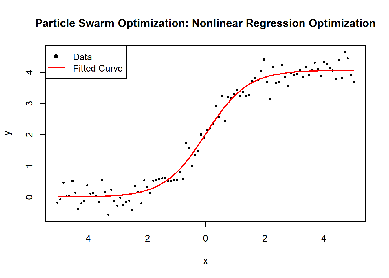
Figure 6.17: Particle Swarm Optimization: Nonlinear Regression Optimization
6.2.3.5 Evolutionary Strategies
Evolutionary Strategies (ES) are a class of evolutionary optimization algorithms that improve solutions by mutating and selecting individuals based on fitness. Unlike Genetic Algorithm, ES focuses on self-adaptive mutation rates and selection pressure rather than crossover. This makes ES particularly robust for continuous optimization problems like nonlinear regression.
ES is particularly useful when:
The function is complex, noisy, or lacks smooth gradients.
Gradient-based methods fail due to non-differentiability.
An adaptive approach to exploration and exploitation is needed.
The goal of ES is to find an optimal solution \(\hat{\theta}\) that minimizes an objective function:
\[ \hat{\theta} = \arg\min_{\theta} SSE(\theta), \]
where:
\[ SSE(\theta) = \sum_{i=1}^{n} (y_i - f(x_i; \theta))^2. \]
1. Population Representation
Each individual is a solution \(\theta_i\) in the parameter space:
\[ \theta_i = (\theta_{i1}, \theta_{i2}, \theta_{i3}). \]
The population consists of multiple individuals, each representing different candidate parameters.
2. Mutation
New candidate solutions are generated by adding random noise:
\[ \theta'_i = \theta_i + \sigma \mathcal{N}(0, I), \]
where:
\(\sigma\) is the mutation step size, which adapts over time.
\(\mathcal{N}(0, I)\) is a standard normal distribution.
3. Selection
ES employs \((\mu, \lambda)\)-selection:
\((\mu, \lambda)\)-ES: Select the best \(\mu\) solutions from \(\lambda\) offspring.
\((\mu + \lambda)\)-ES: Combine parents and offspring, selecting the top \(\mu\).
4. Step-Size Adaptation
Mutation strength \(\sigma\) self-adapts using the 1/5 success rule:
\[ \sigma_{t+1} = \begin{cases} \sigma_t / c, & \text{if success rate } > 1/5 \\ \sigma_t \cdot c, & \text{if success rate } < 1/5 \end{cases} \]
where \(c > 1\) is a scaling factor.
Evolutionary Strategies Algorithm
- Initialize a population of \(\lambda\) solutions with random parameters.
- Set mutation step size \(\sigma\).
- Repeat for max iterations:
- Generate \(\lambda\) offspring by mutating parent solutions.
- Evaluate fitness (SSE) of each offspring.
- Select the best \(\mu\) solutions for the next generation.
- Adapt mutation step size based on success rate.
- Return the best solution found.
# Load required library
library(DEoptim)

# Define a numerically stable logistic function
safe_exp <- function(x) {
    return(ifelse(x > 700, Inf, exp(pmin(x, 700))))  # Prevent overflow
}

# Define the logistic growth model
nonlinear_model <- function(theta, x) {
    return(theta[1] / (1 + safe_exp(-theta[2] * (x - theta[3]))))
}

# Define the Sum of Squared Errors (SSE) function for optimization
sse <- function(theta, x, y) {
    predictions <- nonlinear_model(theta, x)
    return(sum((y - predictions)^2))
}

# Evolutionary Strategies Optimization (Using Differential Evolution)
es_optimization <- function(x, y) {
    # Define fitness function (minimize SSE)
    fitness_function <- function(theta) {
        return(sse(theta, x, y))
    }

    # Set parameter bounds
    lower_bounds <- c(0.1, 0.01, min(x))  # Ensure positive scaling
    upper_bounds <- c(max(y) * 2, 10, max(x))

    # Run Differential Evolution (mimicking ES)
    es_result <- DEoptim(
        fn = fitness_function,
        lower = lower_bounds,
        upper = upper_bounds,
        # 50 individuals, 200 generations, suppress iteration output
        DEoptim.control(NP = 50, itermax = 200, trace = F)
    )

    return(es_result$optim$bestmem)  # Return optimized parameters
}

# Generate synthetic data
set.seed(123)
x <- seq(-5, 5, length.out = 100)
true_theta <- c(4, 1.5, 0)  # True parameters (A, B, C)
y <- nonlinear_model(true_theta, x) + rnorm(length(x), sd = 0.3)

# Run Evolutionary Strategies Optimization
estimated_theta <- es_optimization(x, y)

# Display results
cat("Estimated parameters (A, B, C) using Evolutionary Strategies:\n")
#> Estimated parameters (A, B, C) using Evolutionary Strategies:
print(estimated_theta)
#>       par1       par2       par3
#> 4.06876561 1.42765613 0.01128767
# Plot data and fitted curve
plot(
x, y,
main = "Evolutionary Strategies: Nonlinear Regression Optimization",
pch = 19,
cex = 0.5,
xlab = "x",
ylab = "y"
)
curve(
nonlinear_model(estimated_theta, x),
from = min(x),
to = max(x),
add = TRUE,
col = "red",
lwd = 2
)
legend(
"topleft",
legend = c("Data", "Fitted Curve"),
pch = c(19, NA),
lty = c(NA, 1),
col = c("black", "red")
)
Figure 6.18: Evolutionary Strategies: Nonlinear Regression Optimization
6.2.4 Linearization
6.2.4.1 Taylor Series Approximation
Taylor Series Approximation is a fundamental tool in nonlinear optimization, enabling local approximation of complex functions using polynomial expansions. It is widely used to linearize nonlinear models, facilitate derivative-based optimization, and derive Newton-type methods.
Taylor series approximation is particularly useful when:
A nonlinear function is difficult to compute directly.
Optimization requires local gradient and curvature information.
A simpler, polynomial-based approximation improves computational efficiency.
Given a differentiable function \(f(\theta)\), its Taylor series expansion around a point \(\theta_0\) is:
\[ f(\theta) = f(\theta_0) + f'(\theta_0)(\theta - \theta_0) + \frac{1}{2} f''(\theta_0)(\theta - \theta_0)^2 + \mathcal{O}((\theta - \theta_0)^3). \]
For optimization, we often use:
- First-order approximation (Linear Approximation): \[ f(\theta) \approx f(\theta_0) + f'(\theta_0)(\theta - \theta_0). \]
- Second-order approximation (Quadratic Approximation): \[ f(\theta) \approx f(\theta_0) + f'(\theta_0)(\theta - \theta_0) + \frac{1}{2} f''(\theta_0)(\theta - \theta_0)^2. \]
For gradient-based optimization, we use the Newton-Raphson update:
\[ \theta^{(k+1)} = \theta^{(k)} - [H_f(\theta^{(k)})]^{-1} \nabla f(\theta^{(k)}), \]
where:
\(\nabla f(\theta)\) is the gradient (first derivative),
\(H_f(\theta)\) is the Hessian matrix (second derivative).
For nonlinear regression, we approximate the Sum of Squared Errors (SSE):
\[ SSE(\theta) = \sum_{i=1}^{n} (y_i - f(x_i; \theta))^2. \]
1. First-Order Approximation (Gradient Descent)
The gradient of SSE w.r.t. parameters \(\theta\) is:
\[ \nabla SSE(\theta) = -2 \sum_{i=1}^{n} (y_i - f(x_i; \theta)) \nabla f(x_i; \theta). \]
Using first-order Taylor approximation, we update parameters via gradient descent:
\[ \theta^{(k+1)} = \theta^{(k)} - \alpha \nabla SSE(\theta^{(k)}), \]
where \(\alpha\) is the learning rate.
2. Second-Order Approximation (Newton’s Method)
The Hessian matrix of SSE is:
\[ H_{SSE}(\theta) = 2 \sum_{i=1}^{n} \nabla f(x_i; \theta) \nabla f(x_i; \theta)^T - 2 \sum_{i=1}^{n} (y_i - f(x_i; \theta)) H_f(x_i; \theta). \]
The Newton-Raphson update becomes:
\[ \theta^{(k+1)} = \theta^{(k)} - H_{SSE}(\theta)^{-1} \nabla SSE(\theta). \]
# Load required libraries
library(numDeriv)

# Define a numerically stable logistic function
safe_exp <- function(x) {
    return(ifelse(is.na(x) |
                      x > 700, Inf, exp(pmin(x, 700))))  # Prevent overflow
}

# Define the logistic growth model
nonlinear_model <- function(theta, x) {
    return(theta[1] / (1 + safe_exp(-theta[2] * (x - theta[3]))))
}

# Define the Sum of Squared Errors (SSE) function
sse <- function(theta, x, y) {
    predictions <- nonlinear_model(theta, x)
    return(sum((y - predictions) ^ 2, na.rm = TRUE))  # Avoid NA errors
}

# First-Order Approximation: Gradient Descent Optimization
gradient_descent <-
    function(x,
             y,
             alpha = 0.005,
             tol = 1e-6,
             max_iter = 5000) {
        theta <- c(2, 1, 0)  # Initial guess
        for (i in 1:max_iter) {
            grad_sse <-
                grad(function(t)
                    sse(t, x, y), theta)  # Compute gradient
            theta_new <-
                theta - alpha * grad_sse  # Update parameters

            if (sum(abs(theta_new - theta)) < tol)
                break  # Check convergence
            theta <- theta_new
        }
        return(theta)
    }

# Second-Order Approximation: Newton's Method with Regularization
newton_method <-
    function(x,
             y,
             tol = 1e-6,
             max_iter = 100,
             lambda = 1e-4) {
        theta <- c(2, 1, 0)  # Initial guess
        for (i in 1:max_iter) {
            grad_sse <-
                grad(function(t)
                    sse(t, x, y), theta)  # Compute gradient
            hessian_sse <-
                hessian(function(t)
                    sse(t, x, y), theta)  # Compute Hessian

            # Regularize Hessian to avoid singularity
            hessian_reg <-
                hessian_sse + lambda * diag(length(theta))

            # Ensure Hessian is invertible
            if (is.na(det(hessian_reg)) ||
                det(hessian_reg) < 1e-10) {
                message("Singular Hessian found; increasing regularization.")
                lambda <- lambda * 10  # Increase regularization
                next
            }

            # Newton update
            theta_new <- theta - solve(hessian_reg) %*% grad_sse

            if (sum(abs(theta_new - theta)) < tol)
                break  # Check convergence
            theta <- theta_new
        }
        return(theta)
    }

# Generate synthetic data
set.seed(123)
x <- seq(-5, 5, length.out = 100)
true_theta <- c(4, 1.5, 0)  # True parameters (A, B, C)
y <- nonlinear_model(true_theta, x) + rnorm(length(x), sd = 0.3)

# Run Gradient Descent
estimated_theta_gd <- gradient_descent(x, y)

# Run Newton's Method with Regularization
estimated_theta_newton <- newton_method(x, y)

# Display results
cat("Estimated parameters (A, B, C) using Gradient Descent:\n")
#> Estimated parameters (A, B, C) using Gradient Descent:
print(estimated_theta_gd)
#> [1] 4.06876224 1.42766371 0.01128539

cat("Estimated parameters (A, B, C) using Newton's Method:\n")
#> Estimated parameters (A, B, C) using Newton's Method:
print(estimated_theta_newton)
#>            [,1]
#> [1,] 4.06876368
#> [2,] 1.42766047
#> [3,] 0.01128636
# Plot data and fitted curve
plot(
x,
y,
main = "Taylor Series Approximation: Nonlinear Regression Optimization",
pch = 19,
cex = 0.5,
xlab = "x",
ylab = "y"
)
curve(
nonlinear_model(estimated_theta_gd, x),
from = min(x),
to = max(x),
add = TRUE,
col = "blue",
lwd = 2,
lty = 2 # Dashed line to differentiate Gradient Descent
)
curve(
nonlinear_model(estimated_theta_newton, x),
from = min(x),
to = max(x),
add = TRUE,
col = "red",
lwd = 2
)
legend(
"topleft",
legend = c("Data", "Gradient Descent", "Newton's Method (Regularized)"),
pch = c(19, NA, NA),
lty = c(NA, 2, 1),
col = c("black", "blue", "red")
)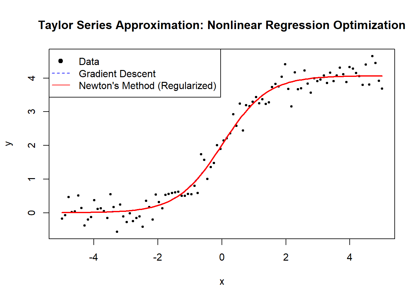
Figure 6.19: Taylor Series Approximation: Nonlinear Regression Optimization
6.2.4.2 Log-Linearization
Log-Linearization is a mathematical technique used to transform nonlinear models into linear models by taking the logarithm of both sides. This transformation simplifies parameter estimation and enables the use of linear regression techniques on originally nonlinear functions.
Log-linearization is particularly useful when:
The model exhibits exponential, power-law, or logistic growth behavior.
Linear regression methods are preferred over nonlinear optimization.
A linearized version provides better interpretability and computational efficiency.
A nonlinear model can often be expressed in the form:
\[ y = f(x; \theta). \]
Applying a log transformation, we obtain:
\[ \log y = g(x; \theta), \]
where \(g(x; \theta)\) is now linear in parameters. We then estimate \(\theta\) using Ordinary Least Squares.
Example 1: Exponential Model
Consider an exponential growth model:
\[ y = A e^{Bx}. \]
Taking the natural logarithm:
\[ \log y = \log A + Bx. \]
This is now linear in \(\log y\), allowing estimation via linear regression.
Example 2: Power Law Model
For a power law function:
\[ y = A x^B. \]
Taking logs:
\[ \log y = \log A + B \log x. \]
Again, this is linearized, making it solvable via OLS regression.
Log-Linearization Algorithm
- Apply the logarithm transformation to the dependent variable.
- Transform the equation into a linear form.
- Use linear regression (OLS) to estimate parameters.
- Convert parameters back to original scale if necessary.
# Load required library
library(stats)

# Generate synthetic data for an exponential model
set.seed(123)
x <- seq(1, 10, length.out = 100)
true_A <- 2
true_B <- 0.3
y <- true_A * exp(true_B * x) + rnorm(length(x), sd = 0.5)

# Apply logarithmic transformation
log_y <- log(y)

# Fit linear regression model
log_linear_model <- lm(log_y ~ x)

# Extract estimated parameters
estimated_B <- coef(log_linear_model)[2]  # Slope in log-space
estimated_A <-
    exp(coef(log_linear_model)[1])  # Intercept (back-transformed)

# Display results
cat("Estimated parameters (A, B) using Log-Linearization:\n")
#> Estimated parameters (A, B) using Log-Linearization:
print(c(estimated_A, estimated_B))
#> (Intercept)           x
#>   2.0012577   0.3001223
# Plot data and fitted curve
plot(
x,
y,
main = "Log-Linearization: Nonlinear Regression Optimization",
pch = 19,
cex = 0.5,
xlab = "x",
ylab = "y"
)
curve(
estimated_A * exp(estimated_B * x),
from = min(x),
to = max(x),
add = TRUE,
col = "red",
lwd = 2
)
legend(
"topleft",
legend = c("Data", "Fitted Log-Linear Model"),
pch = c(19, NA),
lty = c(NA, 1),
col = c("black", "red")
)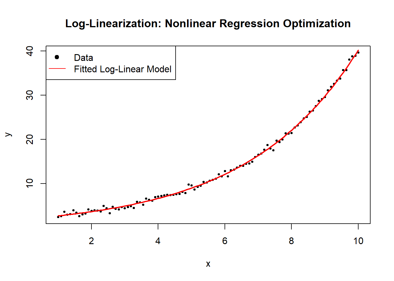
Figure 6.20: Log–Linearization: Nonlinear Regression Optimization
6.2.5 Hybrid
6.2.5.1 Adaptive Levenberg-Marquardt
The Levenberg-Marquardt Algorithm (LMA) is a powerful nonlinear least squares optimization method that adaptively combines:
Gauss-Newton Algorithm for fast convergence near the solution.
Steepest Descent (Gradient Descent) for stability when far from the solution.
The Adaptive Levenberg-Marquardt Algorithm further adjusts the damping parameter \(\tau\) dynamically, making it more efficient in practice.
Given an objective function Sum of Squared Errors (SSE):
\[ SSE(\theta) = \sum_{i=1}^{n} (y_i - f(x_i; \theta))^2. \]
The update rule for LMA is:
\[ \hat{\theta}^{(j+1)} = \hat{\theta}^{(j)} - \alpha_j [\mathbf{F}(\hat{\theta}^{(j)})' \mathbf{F}(\hat{\theta}^{(j)}) + \tau \mathbf{I}_{p \times p}]\frac{\partial \mathbf{Q}(\hat{\theta}^{(j)})}{\partial \theta}. \]
where:
\(\tau\) is the adaptive damping parameter.
\(\mathbf{I}_{p \times p}\) is the identity matrix.
\(\mathbf{F}(\hat{\theta}^{(j)})\) is the Jacobian matrix of partial derivatives.
\(\frac{\partial \mathbf{Q}(\hat{\theta}^{(j)})}{\partial \theta}\) is the gradient vector.
\(\alpha_j\) is the learning rate.
The key adaptation rule for \(\tau\):
If the new step decreases SSE, reduce \(\tau\): \[ \tau \gets \tau / 10. \]
Otherwise, increase \(\tau\) to ensure stability: \[ \tau \gets 10\tau. \]
This adjustment ensures a balance between stability and efficiency.
Adaptive Levenberg-Marquardt Algorithm
- Initialize parameters \(\theta_0\), damping factor \(\tau\).
- Compute Jacobian \(\mathbf{F}(\hat{\theta}^{(j)})\).
- Compute step direction using modified Gauss-Newton update.
- Adjust \(\tau\) dynamically:
- Decrease \(\tau\) if SSE improves.
- Increase \(\tau\) if SSE worsens.
- Repeat until convergence.
# Load required libraries
library(numDeriv)

# Define a numerically stable logistic function
safe_exp <- function(x) {
    return(ifelse(x > 700, Inf, exp(pmin(x, 700))))  # Prevent overflow
}

# Define the logistic growth model
nonlinear_model <- function(theta, x) {
    return(theta[1] / (1 + safe_exp(-theta[2] * (x - theta[3]))))
}

# Define the Sum of Squared Errors (SSE) function
sse <- function(theta, x, y) {
    predictions <- nonlinear_model(theta, x)
    return(sum((y - predictions) ^ 2))
}

# Adaptive Levenberg-Marquardt Optimization
adaptive_lm_optimization <-
    function(x, y, tol = 1e-6, max_iter = 100) {
        theta <- c(2, 1, 0)  # Initial parameter guess
        tau <- 1e-3  # Initial damping parameter
        alpha <- 1  # Step size scaling
        iter <- 0

        while (iter < max_iter) {
            iter <- iter + 1

            # Compute Jacobian numerically
            J <- jacobian(function(t)
                nonlinear_model(t, x), theta)

            # Compute gradient of SSE
            residuals <- y - nonlinear_model(theta, x)
            grad_sse <- -2 * t(J) %*% residuals

            # Compute Hessian approximation
            H <- 2 * t(J) %*% J + tau * diag(length(theta))

            # Compute parameter update step
            delta_theta <- solve(H, grad_sse)

            # Trial step
            theta_new <- theta - alpha * delta_theta

            # Compute SSE for new parameters
            if (sse(theta_new, x, y) < sse(theta, x, y)) {
                # Accept step, decrease tau
                theta <- theta_new
                tau <- tau / 10
            } else {
                # Reject step, increase tau
                tau <- tau * 10
            }

            # Check convergence
            if (sum(abs(delta_theta)) < tol)
                break
        }

        return(theta)
    }

# Generate synthetic data
set.seed(123)
x <- seq(-5, 5, length.out = 100)
true_theta <- c(4, 1.5, 0)  # True parameters (A, B, C)
y <- nonlinear_model(true_theta, x) + rnorm(length(x), sd = 0.3)

# Run Adaptive Levenberg-Marquardt Optimization
estimated_theta <- adaptive_lm_optimization(x, y)

# Display results
cat("Estimated parameters (A, B, C) using Adaptive Levenberg-Marquardt:\n")
#> Estimated parameters (A, B, C) using Adaptive Levenberg-Marquardt:
print(estimated_theta)
#>            [,1]
#> [1,] 4.06876562
#> [2,] 1.42765612
#> [3,] 0.01128767
# Plot data and fitted curve
plot(
x,
y,
main = "Adaptive Levenberg-Marquardt: Nonlinear Regression Optimization",
pch = 19,
cex = 0.5,
xlab = "x",
ylab = "y"
)
curve(
nonlinear_model(estimated_theta, x),
from = min(x),
to = max(x),
add = TRUE,
col = "red",
lwd = 2
)
legend(
"topleft",
legend = c("Data", "Fitted Curve"),
pch = c(19, NA),
lty = c(NA, 1),
col = c("black", "red")
)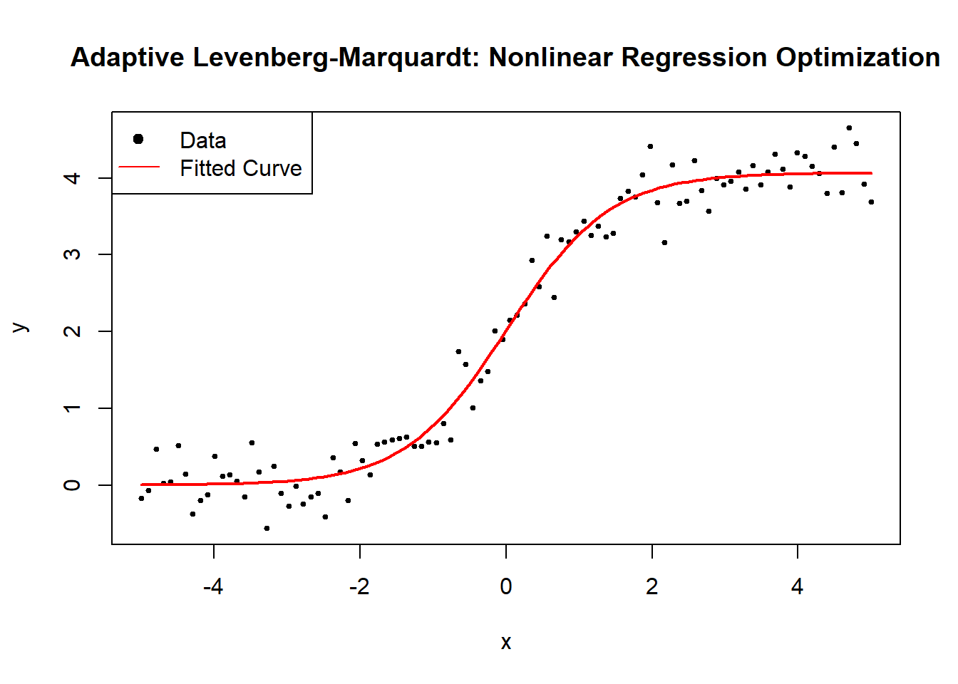
Figure 6.21: Adaptive Levenberg–Marquardt: Nonlinear Regression Optimization
6.2.6 Comparison of Nonlinear Optimizers
# ALL-IN-ONE R SCRIPT COMPARING MULTIPLE NONLINEAR-REGRESSION OPTIMIZERS
library(minpack.lm) # nlsLM (Levenberg-Marquardt)
library(dfoptim) # Powell (nmk), Hooke-Jeeves
library(nloptr) # trust-region reflective
library(GA) # genetic algorithm
library(DEoptim) # differential evolution
library(GenSA) # simulated annealing
library(pso) # particle swarm
library(MASS) # for ginv fallback
library(microbenchmark)
library(ggplot2)
library(dplyr)
# -- 1) DEFINE MODELS (SIMPLE VS COMPLEX) ---
# 3-parameter logistic
f_logistic <- function(theta, x) {
A <- theta[1]
B <- theta[2]
C <- theta[3]
A / (1 + exp(-B * (x - C)))
}
sse_logistic <-
function(theta, x, y)
sum((y - f_logistic(theta, x)) ^ 2)
# 4-parameter "extended" model
f_complex <- function(theta, x) {
A <- theta[1]
B <- theta[2]
C <- theta[3]
D <- theta[4]
A / (1 + exp(-B * (x - C))) + D * exp(-0.5 * x)
}
sse_complex <-
function(theta, x, y)
sum((y - f_complex(theta, x)) ^ 2)
# Generate synthetic data
set.seed(123)
n <- 100
x_data <- seq(-5, 5, length.out = n)
# "simple" scenario
true_theta_simple <- c(4, 1.5, 0)
y_data_simple <-
f_logistic(true_theta_simple, x_data) + rnorm(n, sd = 0.3)
# "complex" scenario
true_theta_complex <- c(4, 1.2, -1, 0.5)
y_data_complex <-
f_complex(true_theta_complex, x_data) + rnorm(n, sd = 0.3)
# -- 2) OPTIMIZERS (EXCEPT BISECTION) ----
#
# All methods share signature:
# FUN(par, x, y, sse_fn, model_fn, lower=NULL, upper=NULL, ...)
# Some do not strictly use lower/upper if unconstrained.
# 2.1 Gauss–Newton
gauss_newton_fit <- function(par,
x,
y,
sse_fn,
model_fn,
lower = NULL,
upper = NULL,
max_iter = 100,
tol = 1e-6)
{
theta <- par
for (iter in seq_len(max_iter)) {
eps <- 1e-6
nP <- length(theta)
Fmat <- matrix(0, nrow = length(x), ncol = nP)
for (p in seq_len(nP)) {
pert <- theta
pert[p] <- pert[p] + eps
Fmat[, p] <-
(model_fn(pert, x) - model_fn(theta, x)) / eps
}
r <- y - model_fn(theta, x)
delta <- tryCatch(
solve(t(Fmat) %*% Fmat, t(Fmat) %*% r),
error = function(e) {
# fallback to pseudoinverse
MASS::ginv(t(Fmat) %*% Fmat) %*% (t(Fmat) %*% r)
}
)
theta_new <- theta + delta
if (sum(abs(theta_new - theta)) < tol)
break
theta <- theta_new
}
theta
}
# 2.2 Modified Gauss-Newton (with step halving)
modified_gauss_newton_fit <- function(par,
x,
y,
sse_fn,
model_fn,
lower = NULL,
upper = NULL,
max_iter = 100,
tol = 1e-6)
{
theta <- par
for (iter in seq_len(max_iter)) {
eps <- 1e-6
nP <- length(theta)
Fmat <- matrix(0, nrow = length(x), ncol = nP)
for (p in seq_len(nP)) {
pert <- theta
pert[p] <- pert[p] + eps
Fmat[, p] <-
(model_fn(pert, x) - model_fn(theta, x)) / eps
}
r <- y - model_fn(theta, x)
lhs <- t(Fmat) %*% Fmat
rhs <- t(Fmat) %*% r
delta <- tryCatch(
solve(lhs, rhs),
error = function(e)
MASS::ginv(lhs) %*% rhs
)
sse_old <- sse_fn(theta, x, y)
alpha <- 1
for (k in 1:10) {
new_sse <- sse_fn(theta + alpha * delta, x, y)
if (new_sse < sse_old)
break
alpha <- alpha / 2
}
theta_new <- theta + alpha * delta
if (sum(abs(theta_new - theta)) < tol)
break
theta <- theta_new
}
theta
}
# 2.3 Steepest Descent (Gradient Descent)
steepest_descent_fit <- function(par,
x,
y,
sse_fn,
model_fn,
lower = NULL,
upper = NULL,
lr = 0.001,
max_iter = 5000,
tol = 1e-6)
{
theta <- par
for (iter in seq_len(max_iter)) {
eps <- 1e-6
f0 <- sse_fn(theta, x, y)
grad <- numeric(length(theta))
for (p in seq_along(theta)) {
pert <- theta
pert[p] <- pert[p] + eps
grad[p] <- (sse_fn(pert, x, y) - f0) / eps
}
theta_new <- theta - lr * grad
if (sum(abs(theta_new - theta)) < tol)
break
theta <- theta_new
}
theta
}
# 2.4 Levenberg–Marquardt (nlsLM)
lm_fit <- function(par,
x,
y,
sse_fn,
model_fn,
lower = NULL,
upper = NULL,
form = c("simple", "complex"))
{
form <- match.arg(form)
if (form == "simple") {
fit <- nlsLM(y ~ A / (1 + exp(-B * (x - C))),
start = list(A = par[1],
B = par[2],
C = par[3]))
} else {
fit <- nlsLM(y ~ A / (1 + exp(-B * (x - C))) + D * exp(-0.5 * x),
start = list(
A = par[1],
B = par[2],
C = par[3],
D = par[4]
))
}
coef(fit)
}
# 2.5 Newton–Raphson (with numeric Hessian, fallback if singular)
newton_raphson_fit <- function(par,
x,
y,
sse_fn,
model_fn,
lower = NULL,
upper = NULL,
max_iter = 50,
tol = 1e-6)
{
theta <- par
for (i in seq_len(max_iter)) {
eps <- 1e-6
f0 <- sse_fn(theta, x, y)
grad <- numeric(length(theta))
for (p in seq_along(theta)) {
pert <- theta
pert[p] <- pert[p] + eps
grad[p] <- (sse_fn(pert, x, y) - f0) / eps
}
Hess <- matrix(0, length(theta), length(theta))
for (p in seq_along(theta)) {
pert_p <- theta
pert_p[p] <- pert_p[p] + eps
f_p <- sse_fn(pert_p, x, y)
for (q in seq_along(theta)) {
pert_q <- pert_p
pert_q[q] <- pert_q[q] + eps
Hess[p, q] <- (sse_fn(pert_q, x, y) -
f_p - (f0 - sse_fn(theta, x, y))) / (eps ^
2)
}
}
delta <- tryCatch(
solve(Hess, grad),
error = function(e)
MASS::ginv(Hess) %*% grad
)
theta_new <- theta - delta
if (sum(abs(theta_new - theta)) < tol)
break
theta <- theta_new
}
theta
}
# 2.6 Quasi–Newton (BFGS via optim)
quasi_newton_fit <- function(par,
x,
y,
sse_fn,
model_fn,
lower = NULL,
upper = NULL)
{
fn <- function(pp)
sse_fn(pp, x, y)
res <- optim(par, fn, method = "BFGS")
res$par
}
# 2.7 Trust-region reflective (nloptr)
trust_region_fit <- function(par,
x,
y,
sse_fn,
model_fn,
lower = NULL,
upper = NULL)
{
# numeric gradient
grad_numeric <- function(pp, eps = 1e-6) {
g <- numeric(length(pp))
f0 <- sse_fn(pp, x, y)
for (i in seq_along(pp)) {
p2 <- pp
p2[i] <- p2[i] + eps
g[i] <- (sse_fn(p2, x, y) - f0) / eps
}
g
}
eval_f <- function(pp) {
val <- sse_fn(pp, x, y)
gr <- grad_numeric(pp)
list(objective = val, gradient = gr)
}
lb <- if (is.null(lower))
rep(-Inf, length(par))
else
lower
ub <- if (is.null(upper))
rep(Inf, length(par))
else
upper
res <- nloptr(
x0 = par,
eval_f = eval_f,
lb = lb,
ub = ub,
opts = list(
algorithm = "NLOPT_LD_TNEWTON",
maxeval = 500,
xtol_rel = 1e-6
)
)
res$solution
}
# 2.8 Grid search
grid_search_fit <- function(par,
x,
y,
sse_fn,
model_fn,
lower = NULL,
upper = NULL,
grid_defs = NULL)
{
if (is.null(grid_defs))
stop("Must provide grid_defs for multi-parameter grid search.")
g <- expand.grid(grid_defs)
g$SSE <-
apply(g, 1, function(rowp)
sse_fn(as.numeric(rowp), x, y))
best_idx <- which.min(g$SSE)
as.numeric(g[best_idx, seq_along(grid_defs)])
}
# 2.9 Nelder-Mead
nelder_mead_fit <- function(par,
x,
y,
sse_fn,
model_fn,
lower = NULL,
upper = NULL)
{
fn <- function(pp)
sse_fn(pp, x, y)
res <- optim(par, fn, method = "Nelder-Mead")
res$par
}
# 2.10 Powell’s method (dfoptim::nmk for unconstrained)
powell_fit <-
function(par,
x,
y,
sse_fn,
model_fn,
lower = NULL,
upper = NULL) {
fn <- function(pp)
sse_fn(pp, x, y)
dfoptim::nmk(par, fn)$par
}
# 2.11 Hooke-Jeeves (dfoptim::hjkb)
hooke_jeeves_fit <-
function(par,
x,
y,
sse_fn,
model_fn,
lower = NULL,
upper = NULL) {
fn <- function(pp)
sse_fn(pp, x, y)
dfoptim::hjkb(par, fn)$par
}
# 2.12 Random Search
random_search_fit <- function(par,
x,
y,
sse_fn,
model_fn,
lower,
upper,
max_iter = 2000,
...)
{
best_par <- NULL
best_sse <- Inf
dimp <- length(lower)
for (i in seq_len(max_iter)) {
candidate <- runif(dimp, min = lower, max = upper)
val <- sse_fn(candidate, x, y)
if (val < best_sse) {
best_sse <- val
best_par <- candidate
}
}
best_par
}
# 2.13 Differential Evolution (DEoptim)
diff_evo_fit <- function(par,
x,
y,
sse_fn,
model_fn,
lower,
upper,
max_iter = 100,
...)
{
fn <- function(v)
sse_fn(v, x, y)
out <- DEoptim(fn,
lower = lower,
upper = upper,
DEoptim.control(NP = 50, itermax = max_iter, trace = F))
out$optim$bestmem
}
# 2.14 Simulated Annealing (GenSA)
sim_anneal_fit <- function(par,
x,
y,
sse_fn,
model_fn,
lower = NULL,
upper = NULL,
...)
{
fn <- function(pp)
sse_fn(pp, x, y)
lb <- if (is.null(lower))
rep(-Inf, length(par))
else
lower
ub <- if (is.null(upper))
rep(Inf, length(par))
else
upper
# GenSA requires: GenSA(par, fn, lower, upper, control=list(...))
out <-
GenSA(
par,
fn,
lower = lb,
upper = ub,
control = list(max.call = 10000)
)
out$par
}
# 2.15 Genetic Algorithm (GA)
genetic_fit <- function(par,
x,
y,
sse_fn,
model_fn,
lower,
upper,
max_iter = 100,
...)
{
fitness_fun <- function(pp)
- sse_fn(pp, x, y)
gares <- ga(
type = "real-valued",
fitness = fitness_fun,
lower = lower,
upper = upper,
popSize = 50,
maxiter = max_iter,
run = 50
)
gares@solution[1,]
}
# 2.16 Particle Swarm (pso)
particle_swarm_fit <- function(par,
x,
y,
sse_fn,
model_fn,
lower,
upper,
max_iter = 100,
...)
{
fn <- function(pp)
sse_fn(pp, x, y)
res <- psoptim(
par = (lower + upper) / 2,
fn = fn,
lower = lower,
upper = upper,
control = list(maxit = max_iter)
)
res$par
}
# -- 3) RUN METHOD WRAPPER ---
run_method <- function(method_name,
FUN,
par_init,
x,
y,
sse_fn,
model_fn,
lower = NULL,
upper = NULL,
...)
{
mb <- microbenchmark(result = {
out <- FUN(par_init, x, y, sse_fn, model_fn, lower, upper, ...)
out
}, times = 1)
final_par <-
FUN(par_init, x, y, sse_fn, model_fn, lower, upper, ...)
if (is.null(final_par)) {
# e.g. placeholders that return NULL
return(data.frame(
Method = method_name,
Parameters = "N/A",
SSE = NA,
Time_ms = NA
))
}
data.frame(
Method = method_name,
Parameters = paste(round(final_par, 4), collapse = ", "),
SSE = round(sse_fn(final_par, x, y), 6),
Time_ms = median(mb$time) / 1e6
)
}
# -- 4) MASTER FUNCTION TO COMPARE ALL METHODS (SIMPLE / COMPLEX) ---
compare_all_methods <- function(is_complex = FALSE) {
if (!is_complex) {
# SIMPLE (3-param logistic)
x <- x_data
y <- y_data_simple
sse_fn <- sse_logistic
model_fn <- f_logistic
init_par <- c(3, 1, 0.5)
grid_defs <- list(
A = seq(2, 6, length.out = 10),
B = seq(0.5, 2, length.out = 10),
C = seq(-1, 1, length.out = 10)
)
lower <- c(1, 0.1,-3)
upper <- c(6, 3, 3)
lm_form <- "simple"
} else {
# COMPLEX (4-param model)
x <- x_data
y <- y_data_complex
sse_fn <- sse_complex
model_fn <- f_complex
init_par <- c(3, 1,-0.5, 0.2)
grid_defs <- list(
A = seq(2, 6, length.out = 8),
B = seq(0.5, 2, length.out = 8),
C = seq(-2, 2, length.out = 8),
D = seq(0, 2, length.out = 8)
)
lower <- c(1, 0.1,-3, 0)
upper <- c(6, 3, 3, 2)
lm_form <- "complex"
}
# RUN each method
out <- bind_rows(
run_method(
"Gauss-Newton",
gauss_newton_fit,
init_par,
x,
y,
sse_fn,
model_fn
),
run_method(
"Modified Gauss-Newton",
modified_gauss_newton_fit,
init_par,
x,
y,
sse_fn,
model_fn
),
run_method(
"Steepest Descent",
steepest_descent_fit,
init_par,
x,
y,
sse_fn,
model_fn
),
run_method(
"Levenberg-Marquardt (nlsLM)",
lm_fit,
init_par,
x,
y,
sse_fn,
model_fn,
form = lm_form
),
run_method(
"Newton-Raphson",
newton_raphson_fit,
init_par,
x,
y,
sse_fn,
model_fn
),
run_method(
"Quasi-Newton (BFGS)",
quasi_newton_fit,
init_par,
x,
y,
sse_fn,
model_fn
),
run_method(
"Trust-region Reflective",
trust_region_fit,
init_par,
x,
y,
sse_fn,
model_fn,
lower,
upper
),
run_method(
"Grid Search",
grid_search_fit,
NULL,
x,
y,
sse_fn,
model_fn,
grid_defs = grid_defs
),
run_method(
"Nelder-Mead",
nelder_mead_fit,
init_par,
x,
y,
sse_fn,
model_fn
),
run_method("Powell's method",
powell_fit,
init_par,
x,
y,
sse_fn,
model_fn),
run_method(
"Hooke-Jeeves",
hooke_jeeves_fit,
init_par,
x,
y,
sse_fn,
model_fn
),
run_method(
"Random Search",
random_search_fit,
NULL,
x,
y,
sse_fn,
model_fn,
lower,
upper,
max_iter = 1000
),
run_method(
"Differential Evolution",
diff_evo_fit,
NULL,
x,
y,
sse_fn,
model_fn,
lower,
upper,
max_iter = 50
),
run_method(
"Simulated Annealing",
sim_anneal_fit,
init_par,
x,
y,
sse_fn,
model_fn,
lower,
upper
),
run_method(
"Genetic Algorithm",
genetic_fit,
NULL,
x,
y,
sse_fn,
model_fn,
lower,
upper,
max_iter = 50
),
run_method(
"Particle Swarm",
particle_swarm_fit,
NULL,
x,
y,
sse_fn,
model_fn,
lower,
upper,
max_iter = 50
)
)
out
}
# -- 5) RUN & VISUALIZE ----
# Compare "simple" logistic (3 params)
results_simple <- compare_all_methods(is_complex = FALSE)
results_simple$Problem <- "Simple"
# Compare "complex" (4 params)
results_complex <- compare_all_methods(is_complex = TRUE)
results_complex$Problem <- "Complex"
# Combine
all_results <- rbind(results_simple, results_complex)
# print(all_results)
# DT::datatable(all_results)# Example: SSE by method & problem
ggplot(all_results, aes(x = Method, y = log(SSE), fill = Problem)) +
geom_bar(stat = "identity", position = "dodge") +
theme_minimal(base_size = 11) +
labs(title = "Comparison of SSE by Method and Problem Complexity",
x = "", y = "Log(Sum of Squared Errors)") +
theme(axis.text.x = element_text(angle = 45, hjust = 1))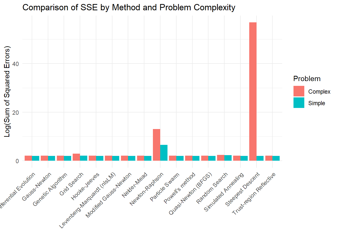
Figure 6.22: Comparison of SSE by Method and Problem Complexity
# Example: Time (ms) by method & problem
ggplot(all_results, aes(x = Method, y = Time_ms, fill = Problem)) +
  geom_bar(stat = "identity", position = "dodge") +
  theme_minimal(base_size = 11) +
  labs(title = "Comparison of Computation Time by Method and Problem Complexity",
       x = "", y = "Time (ms)") +
  theme(axis.text.x = element_text(angle = 45, hjust = 1))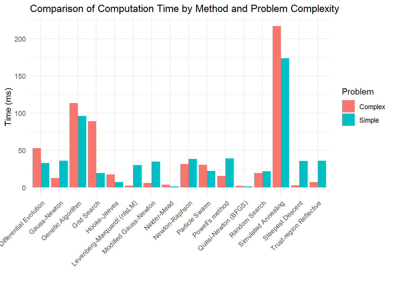
Figure 6.23: Comparison of Computation Time by Method and Problem Complexity