2.5 Data Manipulation

# Load required packages
library(tidyverse)
library(lubridate)

# -----------------------------
# Data Structures in R
# -----------------------------

# Create vectors
x <- c(1, 4, 23, 4, 45)
n <- c(1, 3, 5)
g <- c("M", "M", "F")

# Create a data frame
df <- data.frame(n, g)
df  # View the data frame
#>   n g
#> 1 1 M
#> 2 3 M
#> 3 5 F
str(df)  # Check its structure
#> 'data.frame':    3 obs. of  2 variables:
#>  $ n: num  1 3 5
#>  $ g: chr  "M" "M" "F"

# Using tibble for cleaner outputs
df <- tibble(n, g)
df  # View the tibble
#> # A tibble: 3 × 2
#>       n g    
#>   <dbl> <chr>
#> 1     1 M    
#> 2     3 M    
#> 3     5 F
str(df)
#> tibble [3 × 2] (S3: tbl_df/tbl/data.frame)
#>  $ n: num [1:3] 1 3 5
#>  $ g: chr [1:3] "M" "M" "F"

# Create a list
lst <- list(x, n, g, df)
lst  # Display the list
#> [[1]]
#> [1]  1  4 23  4 45
#> 
#> [[2]]
#> [1] 1 3 5
#> 
#> [[3]]
#> [1] "M" "M" "F"
#> 
#> [[4]]
#> # A tibble: 3 × 2
#>       n g    
#>   <dbl> <chr>
#> 1     1 M    
#> 2     3 M    
#> 3     5 F

# Name list elements
lst2 <- list(num = x, size = n, sex = g, data = df)
lst2  # Named list elements are easier to reference
#> $num
#> [1]  1  4 23  4 45
#> 
#> $size
#> [1] 1 3 5
#> 
#> $sex
#> [1] "M" "M" "F"
#> 
#> $data
#> # A tibble: 3 × 2
#>       n g    
#>   <dbl> <chr>
#> 1     1 M    
#> 2     3 M    
#> 3     5 F

# Another list example with numeric vectors
lst3 <- list(
  x = c(1, 3, 5, 7),
  y = c(2, 2, 2, 4, 5, 5, 5, 6),
  z = c(22, 3, 3, 3, 5, 10)
)
lst3
#> $x
#> [1] 1 3 5 7
#> 
#> $y
#> [1] 2 2 2 4 5 5 5 6
#> 
#> $z
#> [1] 22  3  3  3  5 10

# Find means of list elements
# One at a time
mean(lst3$x)
#> [1] 4
mean(lst3$y)
#> [1] 3.875
mean(lst3$z)
#> [1] 7.666667

# Using lapply to calculate means
lapply(lst3, mean)
#> $x
#> [1] 4
#> 
#> $y
#> [1] 3.875
#> 
#> $z
#> [1] 7.666667

# Simplified output with sapply
sapply(lst3, mean)
#>        x        y        z 
#> 4.000000 3.875000 7.666667

# Tidyverse alternative: map() function
map(lst3, mean)
#> $x
#> [1] 4
#> 
#> $y
#> [1] 3.875
#> 
#> $z
#> [1] 7.666667

# Tidyverse with numeric output: map_dbl()
map_dbl(lst3, mean)
#>        x        y        z 
#> 4.000000 3.875000 7.666667

# -----------------------------
# Binding Data Frames
# -----------------------------

# Create tibbles for demonstration
dat01 <- tibble(x = 1:5, y = 5:1)
dat02 <- tibble(x = 10:16, y = x / 2)
dat03 <- tibble(z = runif(5))  # 5 random numbers from (0, 1)

# Row binding
bind_rows(dat01, dat02, dat01)
#> # A tibble: 17 × 2
#>        x     y
#>    <int> <dbl>
#>  1     1   5  
#>  2     2   4  
#>  3     3   3  
#>  4     4   2  
#>  5     5   1  
#>  6    10   5  
#>  7    11   5.5
#>  8    12   6  
#>  9    13   6.5
#> 10    14   7  
#> 11    15   7.5
#> 12    16   8  
#> 13     1   5  
#> 14     2   4  
#> 15     3   3  
#> 16     4   2  
#> 17     5   1

# Add a new identifier column with .id
bind_rows(dat01, dat02, .id = "id")
#> # A tibble: 12 × 3
#>    id        x     y
#>    <chr> <int> <dbl>
#>  1 1         1   5  
#>  2 1         2   4  
#>  3 1         3   3  
#>  4 1         4   2  
#>  5 1         5   1  
#>  6 2        10   5  
#>  7 2        11   5.5
#>  8 2        12   6  
#>  9 2        13   6.5
#> 10 2        14   7  
#> 11 2        15   7.5
#> 12 2        16   8

# Use named inputs for better identification
bind_rows("dat01" = dat01, "dat02" = dat02, .id = "id")
#> # A tibble: 12 × 3
#>    id        x     y
#>    <chr> <int> <dbl>
#>  1 dat01     1   5  
#>  2 dat01     2   4  
#>  3 dat01     3   3  
#>  4 dat01     4   2  
#>  5 dat01     5   1  
#>  6 dat02    10   5  
#>  7 dat02    11   5.5
#>  8 dat02    12   6  
#>  9 dat02    13   6.5
#> 10 dat02    14   7  
#> 11 dat02    15   7.5
#> 12 dat02    16   8

# Bind a list of data frames
list01 <- list("dat01" = dat01, "dat02" = dat02)
bind_rows(list01, .id = "source")
#> # A tibble: 12 × 3
#>    source     x     y
#>    <chr>  <int> <dbl>
#>  1 dat01      1   5  
#>  2 dat01      2   4  
#>  3 dat01      3   3  
#>  4 dat01      4   2  
#>  5 dat01      5   1  
#>  6 dat02     10   5  
#>  7 dat02     11   5.5
#>  8 dat02     12   6  
#>  9 dat02     13   6.5
#> 10 dat02     14   7  
#> 11 dat02     15   7.5
#> 12 dat02     16   8

# Column binding
bind_cols(dat01, dat03)
#> # A tibble: 5 × 3
#>       x     y     z
#>   <int> <int> <dbl>
#> 1     1     5 0.265
#> 2     2     4 0.410
#> 3     3     3 0.780
#> 4     4     2 0.926
#> 5     5     1 0.501

# -----------------------------
# String Manipulation
# -----------------------------

names <- c("Ford, MS", "Jones, PhD", "Martin, Phd", "Huck, MA, MLS")

# Remove everything after the first comma
str_remove(names, pattern = ", [[:print:]]+")
#> [1] "Ford"   "Jones"  "Martin" "Huck"

# Explanation: [[:print:]]+ matches one or more printable characters

# -----------------------------
# Reshaping Data
# -----------------------------

# Wide format data
wide <- data.frame(
  name = c("Clay", "Garrett", "Addison"),
  test1 = c(78, 93, 90),
  test2 = c(87, 91, 97),
  test3 = c(88, 99, 91)
)

# Long format data
long <- data.frame(
  name = rep(c("Clay", "Garrett", "Addison"), each = 3),
  test = rep(1:3, 3),
  score = c(78, 87, 88, 93, 91, 99, 90, 97, 91)
)

# Summary statistics
aggregate(score ~ name, data = long, mean)  # Mean score per student
#>      name    score
#> 1 Addison 92.66667
#> 2    Clay 84.33333
#> 3 Garrett 94.33333
aggregate(score ~ test, data = long, mean)  # Mean score per test
#>   test    score
#> 1    1 87.00000
#> 2    2 91.66667
#> 3    3 92.66667

# Line plot of scores over tests
ggplot(long,
       aes(
           x = factor(test),
           y = score,
           color = name,
           group = name
       )) +
    geom_point() +
    geom_line() +
    xlab("Test") +
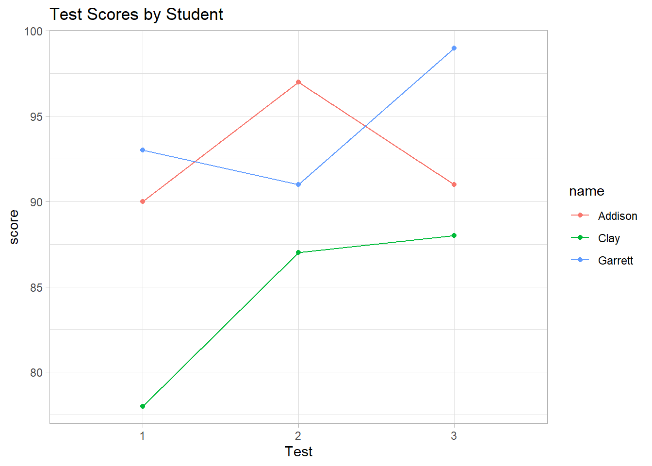
    ggtitle("Test Scores by Student")

# Reshape wide to long
pivot_longer(wide, test1:test3, names_to = "test", values_to = "score")
#> # A tibble: 9 × 3
#>   name    test  score
#>   <chr>   <chr> <dbl>
#> 1 Clay    test1    78
#> 2 Clay    test2    87
#> 3 Clay    test3    88
#> 4 Garrett test1    93
#> 5 Garrett test2    91
#> 6 Garrett test3    99
#> 7 Addison test1    90
#> 8 Addison test2    97
#> 9 Addison test3    91

# Use names_prefix to clean column names
pivot_longer(
    wide,
    -name,
    names_to = "test",
    values_to = "score",
    names_prefix = "test"
)
#> # A tibble: 9 × 3
#>   name    test  score
#>   <chr>   <chr> <dbl>
#> 1 Clay    1        78
#> 2 Clay    2        87
#> 3 Clay    3        88
#> 4 Garrett 1        93
#> 5 Garrett 2        91
#> 6 Garrett 3        99
#> 7 Addison 1        90
#> 8 Addison 2        97
#> 9 Addison 3        91

# Reshape long to wide with explicit id_cols argument
pivot_wider(
  long,
  id_cols = name, 
  names_from = test,
  values_from = score
)
#> # A tibble: 3 × 4
#>   name      `1`   `2`   `3`
#>   <chr>   <dbl> <dbl> <dbl>
#> 1 Clay       78    87    88
#> 2 Garrett    93    91    99
#> 3 Addison    90    97    91

# Add a prefix to the resulting columns
pivot_wider(
  long,
  id_cols = name,  
  names_from = test,
  values_from = score,
  names_prefix = "test"
)
#> # A tibble: 3 × 4
#>   name    test1 test2 test3
#>   <chr>   <dbl> <dbl> <dbl>
#> 1 Clay       78    87    88
#> 2 Garrett    93    91    99
#> 3 Addison    90    97    91

The verbs of data manipulation

• select: selecting (or not selecting) columns based on their names (eg: select columns Q1 through Q25)
• slice: selecting (or not selecting) rows based on their position (eg: select rows 1:10)
• mutate: add or derive new columns (or variables) based on existing columns (eg: create a new column that expresses measurement in cm based on existing measure in inches)
• rename: rename variables or change column names (eg: change “GraduationRate100” to “grad100”)
• filter: selecting rows based on a condition (eg: all rows where gender = Male)
• arrange: ordering rows based on variable(s) numeric or alphabetical order (eg: sort in descending order of Income)
• sample: take random samples of data (eg: sample 80% of data to create a “training” set)
• summarize: condense or aggregate multiple values into single summary values (eg: calculate median income by age group)
• group_by: convert a tbl into a grouped tbl so that operations are performed “by group”; allows us to summarize data or apply verbs to data by groups (eg, by gender or treatment)
• the pipe: %>%

  • Use Ctrl + Shift + M (Win) or Cmd + Shift + M (Mac) to enter in RStudio

  • The pipe takes the output of a function and “pipes” into the first argument of the next function.

  • new pipe is |> It should be identical to the old one, except for certain special cases.

• := (Walrus operator): similar to = , but for cases where you want to use the glue package (i.e., dynamic changes in the variable name in the left-hand side)

Writing function in R

Tunneling

{{ (called curly-curly) allows you to tunnel data-variables through arg-variables (i.e., function arguments)

library(tidyverse)
# -----------------------------
# Writing Functions with {{ }}
# -----------------------------

# Define a custom function using {{ }}
get_mean <- function(data, group_var, var_to_mean) {
  data %>%
    group_by({{group_var}}) %>%
    summarize(mean = mean({{var_to_mean}}, na.rm = TRUE))
}

# Apply the function
data("mtcars")
mtcars %>%
  get_mean(group_var = cyl, var_to_mean = mpg)
#> # A tibble: 3 × 2
#>     cyl  mean
#>   <dbl> <dbl>
#> 1     4  26.7
#> 2     6  19.7
#> 3     8  15.1

# Dynamically name the resulting variable
get_mean <- function(data, group_var, var_to_mean, prefix = "mean_of") {
  data %>%
    group_by({{group_var}}) %>%
    summarize("{prefix}_{{var_to_mean}}" := mean({{var_to_mean}}, na.rm = TRUE))
}

# Apply the modified function
mtcars %>%
  get_mean(group_var = cyl, var_to_mean = mpg)
#> # A tibble: 3 × 2
#>     cyl mean_of_mpg
#>   <dbl>       <dbl>
#> 1     4        26.7
#> 2     6        19.7
#> 3     8        15.1