7.4 Poisson Regression
7.4.1 The Poisson Distribution
Poisson regression is used for modeling count data, where the response variable represents the number of occurrences of an event within a fixed period, space, or other unit. The Poisson distribution is defined as:
\[ \begin{aligned} f(Y_i) &= \frac{\mu_i^{Y_i} \exp(-\mu_i)}{Y_i!}, \quad Y_i = 0,1,2, \dots \\ E(Y_i) &= \mu_i \\ \text{Var}(Y_i) &= \mu_i \end{aligned} \] where:
\(Y_i\) is the count variable.
\(\mu_i\) is the expected count for the \(i\)-th observation.
The mean and variance are equal \(E(Y_i) = \text{Var}(Y_i)\), making Poisson regression suitable when variance follows this property.
However, real-world count data often exhibit overdispersion, where the variance exceeds the mean. We will discuss remedies such as Quasi-Poisson and Negative Binomial Regression later.
7.4.2 Poisson Model
We model the expected count \(\mu_i\) as a function of predictors \(\mathbf{x_i}\) and parameters \(\boldsymbol{\theta}\):
\[ \mu_i = f(\mathbf{x_i; \theta}) \]
7.4.3 Link Function Choices
Since \(\mu_i\) must be positive, we often use a log-link function:
\[ θ\log(\mu_i) = \mathbf{x_i' \theta} \]
This ensures that the predicted counts are always non-negative. This is analogous to logistic regression, where we use the logit link for binary outcomes.
Rewriting:
\[ \mu_i = \exp(\mathbf{x_i' \theta}) \] which ensures \(\mu_i > 0\) for all parameter values.
7.4.4 Application: Poisson Regression
We apply Poisson regression to the bioChemists dataset (from the pscl package), which contains information on academic productivity in terms of published articles.
7.4.4.1 Dataset Overview
library(tidyverse)
# Load dataset
data(bioChemists, package = "pscl")

# Rename columns for clarity
bioChemists <- bioChemists %>%
  rename(
    Num_Article = art,
    # Number of articles in last 3 years
    Sex = fem,
    # 1 if female, 0 if male
    Married = mar,
    # 1 if married, 0 otherwise
    Num_Kid5 = kid5,
    # Number of children under age 6
    PhD_Quality = phd,
    # Prestige of PhD program
    Num_MentArticle = ment   # Number of articles by mentor in last 3 years
  )
# Visualize response variable distribution
hist(bioChemists$Num_Article,
breaks = 25,
main = "Number of Articles Published")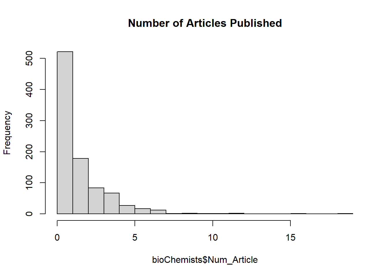
Figure 7.7: Number of Articles Published
The distribution of the number of articles is right-skewed, which suggests a Poisson model may be appropriate.
7.4.4.2 Fitting a Poisson Regression Model
We model the number of articles published (Num_Article) as a function of various predictors.
# Poisson regression model
Poisson_Mod <-
  glm(Num_Article ~ .,
      family = poisson,
      data = bioChemists)

# Summary of the model
summary(Poisson_Mod)
#>
#> Call:
#> glm(formula = Num_Article ~ ., family = poisson, data = bioChemists)
#>
#> Coefficients:
#>                  Estimate Std. Error z value Pr(>|z|)
#> (Intercept)      0.304617   0.102981   2.958   0.0031 **
#> SexWomen        -0.224594   0.054613  -4.112 3.92e-05 ***
#> MarriedMarried   0.155243   0.061374   2.529   0.0114 *
#> Num_Kid5        -0.184883   0.040127  -4.607 4.08e-06 ***
#> PhD_Quality      0.012823   0.026397   0.486   0.6271
#> Num_MentArticle  0.025543   0.002006  12.733  < 2e-16 ***
#> ---
#> Signif. codes:  0 '***' 0.001 '**' 0.01 '*' 0.05 '.' 0.1 ' ' 1
#>
#> (Dispersion parameter for poisson family taken to be 1)
#>
#>     Null deviance: 1817.4  on 914  degrees of freedom
#> Residual deviance: 1634.4  on 909  degrees of freedom
#> AIC: 3314.1
#>
#> Number of Fisher Scoring iterations: 5
Interpretation:
Coefficients are on the log scale, meaning they represent log-rate ratios.
Exponentiating the coefficients gives the rate ratios.
Statistical significance tells us whether each variable has a meaningful impact on publication count.
7.4.4.3 Model Diagnostics: Goodness of Fit
7.4.4.3.1 Pearson’s Chi-Square Test for Overdispersion
We compute the Pearson chi-square statistic to check whether the variance significantly exceeds the mean.
\[ X^2 = \sum \frac{(Y_i - \hat{\mu}_i)^2}{\hat{\mu}_i} \]
# Compute predicted means
Predicted_Means <- predict(Poisson_Mod, type = "response")

# Pearson chi-square test
X2 <-
  sum((bioChemists$Num_Article - Predicted_Means) ^ 2 / Predicted_Means)
X2
#> [1] 1662.547
pchisq(X2, Poisson_Mod$df.residual, lower.tail = FALSE)
#> [1] 7.849882e-47
If p-value is small, overdispersion is present.
Large X² statistic suggests the model may not adequately capture variability.
7.4.4.4 Addressing Overdispersion
7.4.4.4.1 Including Interaction Terms
One possible remedy is to incorporate interaction terms, capturing complex relationships between predictors.
# Adding two-way and three-way interaction terms
Poisson_Mod_All2way <-
  glm(Num_Article ~ . ^ 2, family = poisson, data = bioChemists)
Poisson_Mod_All3way <-
  glm(Num_Article ~ . ^ 3, family = poisson, data = bioChemists)
This may improve model fit, but can lead to overfitting.
7.4.4.4.2 Quasi-Poisson Model (Adjusting for Overdispersion)
A quick fix is to allow the variance to scale by introducing \(\hat{\phi}\):
\[ \text{Var}(Y_i) = \hat{\phi} \mu_i \]
# Estimate dispersion parameter
phi_hat = Poisson_Mod$deviance / Poisson_Mod$df.residual

# Adjusting Poisson model to account for overdispersion
summary(Poisson_Mod, dispersion = phi_hat)
#>
#> Call:
#> glm(formula = Num_Article ~ ., family = poisson, data = bioChemists)
#>
#> Coefficients:
#>                 Estimate Std. Error z value Pr(>|z|)
#> (Intercept)      0.30462    0.13809   2.206  0.02739 *
#> SexWomen        -0.22459    0.07323  -3.067  0.00216 **
#> MarriedMarried   0.15524    0.08230   1.886  0.05924 .
#> Num_Kid5        -0.18488    0.05381  -3.436  0.00059 ***
#> PhD_Quality      0.01282    0.03540   0.362  0.71715
#> Num_MentArticle  0.02554    0.00269   9.496  < 2e-16 ***
#> ---
#> Signif. codes:  0 '***' 0.001 '**' 0.01 '*' 0.05 '.' 0.1 ' ' 1
#>
#> (Dispersion parameter for poisson family taken to be 1.797988)
#>
#>     Null deviance: 1817.4  on 914  degrees of freedom
#> Residual deviance: 1634.4  on 909  degrees of freedom
#> AIC: 3314.1
#>
#> Number of Fisher Scoring iterations: 5
Alternatively, we refit using a Quasi-Poisson model, which adjusts standard errors:
# Quasi-Poisson model
quasiPoisson_Mod <- glm(Num_Article ~ ., family = quasipoisson, data = bioChemists)
summary(quasiPoisson_Mod)
#>
#> Call:
#> glm(formula = Num_Article ~ ., family = quasipoisson, data = bioChemists)
#>
#> Coefficients:
#>                  Estimate Std. Error t value Pr(>|t|)
#> (Intercept)      0.304617   0.139273   2.187 0.028983 *
#> SexWomen        -0.224594   0.073860  -3.041 0.002427 **
#> MarriedMarried   0.155243   0.083003   1.870 0.061759 .
#> Num_Kid5        -0.184883   0.054268  -3.407 0.000686 ***
#> PhD_Quality      0.012823   0.035700   0.359 0.719544
#> Num_MentArticle  0.025543   0.002713   9.415  < 2e-16 ***
#> ---
#> Signif. codes:  0 '***' 0.001 '**' 0.01 '*' 0.05 '.' 0.1 ' ' 1
#>
#> (Dispersion parameter for quasipoisson family taken to be 1.829006)
#>
#>     Null deviance: 1817.4  on 914  degrees of freedom
#> Residual deviance: 1634.4  on 909  degrees of freedom
#> AIC: NA
#>
#> Number of Fisher Scoring iterations: 5
While Quasi-Poisson corrects standard errors, it does not introduce an extra parameter for overdispersion.
7.4.4.4.3 Negative Binomial Regression (Preferred Approach)
A Negative Binomial Regression explicitly models overdispersion by introducing a dispersion parameter \(\theta\):
\[ \text{Var}(Y_i) = \mu_i + \theta \mu_i^2 \]
This extends Poisson regression by allowing the variance to grow quadratically rather than linearly.
# Load MASS package
library(MASS)

# Fit Negative Binomial regression
NegBin_Mod <- glm.nb(Num_Article ~ ., data = bioChemists)

# Model summary
summary(NegBin_Mod)
#>
#> Call:
#> glm.nb(formula = Num_Article ~ ., data = bioChemists, init.theta = 2.264387695,
#>     link = log)
#>
#> Coefficients:
#>                  Estimate Std. Error z value Pr(>|z|)
#> (Intercept)      0.256144   0.137348   1.865 0.062191 .
#> SexWomen        -0.216418   0.072636  -2.979 0.002887 **
#> MarriedMarried   0.150489   0.082097   1.833 0.066791 .
#> Num_Kid5        -0.176415   0.052813  -3.340 0.000837 ***
#> PhD_Quality      0.015271   0.035873   0.426 0.670326
#> Num_MentArticle  0.029082   0.003214   9.048  < 2e-16 ***
#> ---
#> Signif. codes:  0 '***' 0.001 '**' 0.01 '*' 0.05 '.' 0.1 ' ' 1
#>
#> (Dispersion parameter for Negative Binomial(2.2644) family taken to be 1)
#>
#>     Null deviance: 1109.0  on 914  degrees of freedom
#> Residual deviance: 1004.3  on 909  degrees of freedom
#> AIC: 3135.9
#>
#> Number of Fisher Scoring iterations: 1
#>
#>
#>               Theta:  2.264
#>           Std. Err.:  0.271
#>
#>  2 x log-likelihood:  -3121.917
This model is generally preferred over Quasi-Poisson, as it explicitly accounts for heterogeneity in the data.