32.11 Generalized Synthetic Control

The Generalized Synthetic Control (GSC) Method extends the synthetic control approach to accommodate multiple treated units and heterogeneous treatment effects while relaxing the parallel trends assumption required in difference-in-differences. Originally developed by Xu (2017), the GSC method integrates interactive fixed effects models, improving efficiency and robustness in time-series cross-sectional (TSCS) data.

32.11.1 The Problem with Traditional Methods

Traditional causal inference methods such as DID require the parallel trends assumption: $E[Y_{it}(0) | D_i = 1] - E[Y_{it}(0) | D_i = 0] = \text{constant}$ which states that in the absence of treatment, the difference in outcomes between treated and control units would have remained constant over time. However, this assumption often fails due to:

Time-varying unobserved confounders affecting both treatment assignment and outcomes.
Heterogeneous treatment effects across units and over time.
Multiple treatment periods where different units adopt the treatment at different times.

To address these limitations, GSC builds on the interactive fixed effects model, which allows for unit-specific and time-specific latent factors that can capture unobserved confounding trends.

32.11.2 Generalized Synthetic Control Model

Let $Y_{it}$ represent the observed outcome of unit $i$ at time $t$ , and define the potential outcomes framework: $Y_{it}(d) = \mu_{it} + \delta_{it} d + \varepsilon_{it}, \quad d \in \{0,1\}$ where:

$\mu_{it}$ represents the latent factor structure of untreated outcomes.
$\delta_{it}$ is the treatment effect.
$\varepsilon_{it}$ is the idiosyncratic error term.

Under the interactive fixed effects model, we assume that the untreated outcome follows: $\mu_{it} = X_{it} \beta + \lambda_i' f_t$ where:

$X_{it}$ is a vector of observed covariates.
$\beta$ is a vector of unknown coefficients.
$\lambda_i$ represents unit-specific factor loadings.
$f_t$ represents time-specific factors.

The presence of $\lambda_i' f_t$ allows GSC to control for unobserved confounders that vary across time and units, a key advantage over DID and traditional SCM.

32.11.3 Identification and Estimation

To estimate the Average Treatment Effect on the Treated, we define: $\text{ATT}_t = \frac{1}{N_T} \sum_{i \in T} \left[ Y_{it}(1) - Y_{it}(0) \right]$ where $N_T$ is the number of treated units. The challenge is that $Y_{it}(0)$ for treated units is counterfactual and must be estimated.

Step 1: Estimating Factor Loadings and Latent Factors

Using only control units, we estimate the latent factors and factor loadings: $Y_{it} = X_{it} \beta + \lambda_i' f_t + \varepsilon_{it}, \quad i \in C$ which can be rewritten in matrix form: $Y_C = X_C \beta + \Lambda_C F' + E_C.$ The key assumption is that factor loadings and latent factors apply to both treated and control units, ensuring valid counterfactual estimation.

Step 2: Imputing Counterfactual Outcomes

For treated units, we estimate: $\hat{\lambda}_i = (F_0'F_0)^{-1} F_0' (Y_{i,0} - X_{i,0} \beta)$ where $F_0$ and $Y_{i,0}$ denote pre-treatment data. The imputed counterfactuals are then:

$\hat{Y}_{it}(0) = X_{it} \beta + \hat{\lambda}_i' \hat{f}_t.$

32.11.4 Bootstrap Procedure for Standard Errors

A key issue in statistical inference with GSC is the estimation of uncertainty. The standard nonparametric bootstrap is biased due to dependent structures in panel data we adopt the parametric bootstrap from (K. T. Li and Sonnier 2023) to correct for bias.

Corrected Bootstrap Algorithm:

Estimate the IFE Model using control units.
Resample residuals $\hat{\varepsilon}_{it}$ from the fitted model.
Generate new synthetic datasets using: $Y_{it}^* = X_{it} \hat{\beta} + \hat{\lambda}_i' \hat{f}_t + \varepsilon_{it}^*$
Re-estimate the model on resampled data and compute bootstrap confidence intervals.

This approach ensures correct coverage probabilities and avoids bias in standard error estimation.

# Load required package
library(gsynth)

# Example data
data("gsynth")

# Fit Generalized Synthetic Control Model
gsc_model <-
    gsynth(
        Y ~ D + X1 + X2,
        data = simdata,
        parallel = FALSE,
        index = c("id", "time"),
        force = "two-way",
        CV = TRUE,
        r = c(0, 5),
        se = T
    )
#> Cross-validating ... 
#>  r = 0; sigma2 = 1.84865; IC = 1.02023; PC = 1.74458; MSPE = 2.37280
#>  r = 1; sigma2 = 1.51541; IC = 1.20588; PC = 1.99818; MSPE = 1.71743
#>  r = 2; sigma2 = 0.99737; IC = 1.16130; PC = 1.69046; MSPE = 1.14540*
#>  r = 3; sigma2 = 0.94664; IC = 1.47216; PC = 1.96215; MSPE = 1.15032
#>  r = 4; sigma2 = 0.89411; IC = 1.76745; PC = 2.19241; MSPE = 1.21397
#>  r = 5; sigma2 = 0.85060; IC = 2.05928; PC = 2.40964; MSPE = 1.23876
#> 
#>  r* = 2
#> 
#> 
Bootstrapping ...
#> ..

# Summary of results
summary(gsc_model)
#>              Length Class   Mode     
#> Y.dat         1500  -none-  numeric  
#> Y                1  -none-  character
#> D                1  -none-  character
#> X                2  -none-  character
#> W                0  -none-  NULL     
#> index            2  -none-  character
#> id              50  -none-  numeric  
#> time            30  -none-  numeric  
#> obs.missing   1500  -none-  numeric  
#> id.tr            5  -none-  numeric  
#> id.co           45  -none-  numeric  
#> D.tr           150  -none-  numeric  
#> I.tr           150  -none-  numeric  
#> Y.tr           150  -none-  numeric  
#> Y.ct           150  -none-  numeric  
#> Y.co          1350  -none-  numeric  
#> eff            150  -none-  numeric  
#> Y.bar           90  -none-  numeric  
#> att             30  -none-  numeric  
#> att.avg          1  -none-  numeric  
#> force            1  -none-  numeric  
#> sameT0           1  -none-  logical  
#> T                1  -none-  numeric  
#> N                1  -none-  numeric  
#> p                1  -none-  numeric  
#> Ntr              1  -none-  numeric  
#> Nco              1  -none-  numeric  
#> T0               5  -none-  numeric  
#> tr              50  -none-  logical  
#> pre            150  -none-  logical  
#> post           150  -none-  logical  
#> r.cv             1  -none-  numeric  
#> IC               1  -none-  numeric  
#> PC               1  -none-  numeric  
#> beta             2  -none-  numeric  
#> est.co          13  -none-  list     
#> mu               1  -none-  numeric  
#> validX           1  -none-  numeric  
#> sigma2           1  -none-  numeric  
#> res.co        1350  -none-  numeric  
#> MSPE             1  -none-  numeric  
#> CV.out          30  -none-  numeric  
#> niter            1  -none-  numeric  
#> factor          60  -none-  numeric  
#> lambda.co       90  -none-  numeric  
#> lambda.tr       10  -none-  numeric  
#> wgt.implied    225  -none-  numeric  
#> alpha.tr         5  -none-  numeric  
#> alpha.co        45  -none-  numeric  
#> xi              30  -none-  numeric  
#> inference        1  -none-  character
#> est.att        180  -none-  numeric  
#> est.avg          5  -none-  numeric  
#> att.avg.boot   200  -none-  numeric  
#> att.boot      6000  -none-  numeric  
#> eff.boot     30000  -none-  numeric  
#> Dtr.boot     30000  -none-  numeric  
#> Itr.boot     30000  -none-  numeric  
#> beta.boot      400  -none-  numeric  
#> est.beta        10  -none-  numeric  
#> call             9  -none-  call     
#> formula          3  formula call

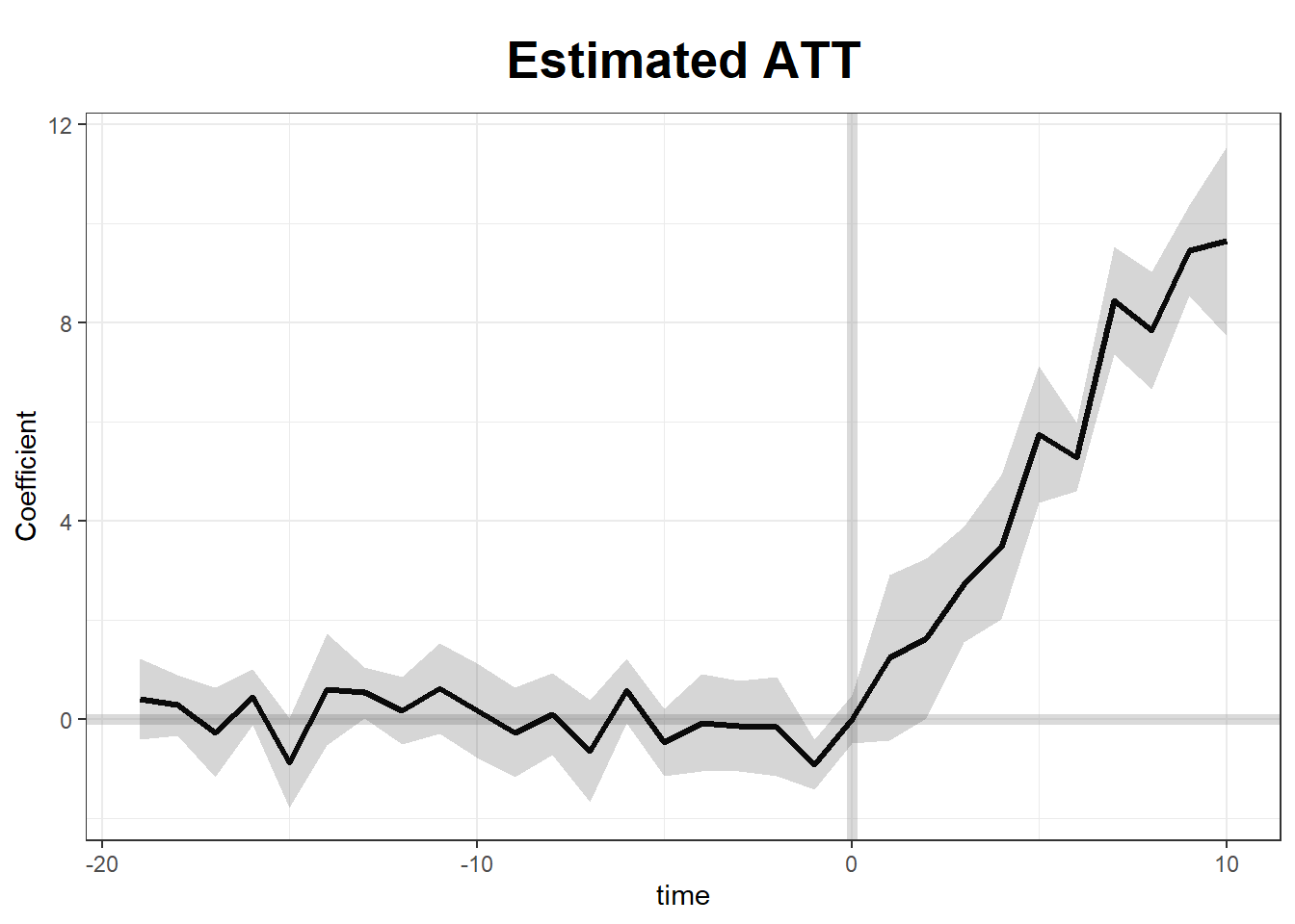
# Visualization
plot(gsc_model)

References

Li, Kathleen T, and Garrett P Sonnier. 2023. “Statistical Inference for the Factor Model Approach to Estimate Causal Effects in Quasi-Experimental Settings.” Journal of Marketing Research 60 (3): 449–72.

Xu, Yiqing. 2017. “Generalized Synthetic Control Method: Causal Inference with Interactive Fixed Effects Models.” Political Analysis 25 (1): 57–76.