15.2 Wrapper Methods (Model-Based Subset Evaluation)
15.2.1 Best Subsets Algorithm
The Best Subsets Algorithm is a systematic method for selecting the best combination of predictors. Unlike exhaustive search, which evaluates all possible subsets of predictors, this algorithm efficiently narrows the search space while guaranteeing the identification of the best subset for each size.
- The algorithm is based on the “leap and bounds” method introduced by (Furnival and Wilson 2000).
- It combines:
- Comparison of SSE: Evaluates models by their Sum of Squared Errors.
- Control over sequence: Optimizes the order in which subset models are computed.
- Guarantees: Finds the best \(m\) subset models within each subset size while reducing computational burden compared to evaluating all possible subsets.
Key Features
- Subset Comparison:
- The algorithm ranks subsets based on a criterion such as \(R^2\), adjusted \(R^2\), AIC, or BIC.
- It evaluates models of varying sizes, starting from 1 predictor to \(p\) predictors.
- Efficiency:
- By leveraging “leap and bounds,” the algorithm avoids evaluating subsets unlikely to yield the best results.
- This reduces the computational cost significantly compared to evaluating \(2^p\) subsets in exhaustive search.
- Output:
- Produces the best subsets for each model size, which can be compared using criteria like AIC, BIC, or PRESS.
# Load the leaps package
library("leaps")

# Simulated data
set.seed(123)
n <- 100
x1 <- rnorm(n)
x2 <- rnorm(n)
x3 <- rnorm(n)
x4 <- rnorm(n)
y <- 5 + 3*x1 - 2*x2 + x3 + rnorm(n, sd=2)

# Prepare data for best subsets model
data <- data.frame(y, x1, x2, x3, x4)

# Perform best subsets model
best_subsets <- regsubsets(y ~ ., data = data, nvmax = 4)

# Summarize results
best_summary <- summary(best_subsets)

# Display model selection metrics
cat("Best Subsets Summary:\n")
#> Best Subsets Summary:
cat("Adjusted R^2:\n", best_summary$adjr2, "\n")
#> Adjusted R^2:
#>  0.3651194 0.69237 0.7400424 0.7374724
cat("Cp:\n", best_summary$cp, "\n")
#> Cp:
#>  140.9971 19.66463 3.060205 5
cat("BIC:\n", best_summary$bic, "\n")
#> BIC:
#>  -37.23673 -106.1111 -119.3802 -114.8383

# Visualize results
plot(best_subsets, scale = "adjr2")
title("Best Subsets: Adjusted R^2")
Interpretation
Model Size:
Examine the metrics for models with 1, 2, 3, and 4 predictors.
Choose the model size that optimizes your preferred metric (e.g., maximized adjusted \(R^2\), minimized BIC).
Model Comparison:
For small datasets, adjusted \(R^2\) is often a reliable criterion.
For larger datasets, use BIC or AIC to avoid overfitting.
Efficiency:
- The algorithm evaluates far fewer models than an exhaustive search while still guaranteeing optimal results for each subset size.
Advantages:
Computationally efficient compared to evaluating all possible subsets.
Guarantees the best subsets for each model size.
Flexibility to use different selection criteria (e.g., \(R^2\), AIC, BIC).
Limitations:
May become computationally intensive for very large \(p\) (e.g., hundreds of predictors).
Assumes linear relationships among predictors and the outcome.
Practical Considerations
When to use Best Subsets?
For datasets with a moderate number of predictors (\(p \leq 20\)).
When you need an optimal solution for each subset size.
Alternatives:
Stepwise Selection: Faster but less reliable.
Regularization Techniques: LASSO and Ridge regression handle large \(p\) and collinearity effectively.
15.2.2 Stepwise Selection Methods
Stepwise selection procedures are iterative methods for selecting predictor variables. These techniques balance model simplicity and predictive accuracy by systematically adding or removing variables based on predefined criteria.
Notes:
- Computer implementations often replace exact F-values with “significance” levels:
- SLE: Significance level to enter.
- SLS: Significance level to stay.
- These thresholds serve as guides rather than strict tests of significance.
Balancing SLE and SLS:
- Large SLE values: May include too many variables, risking overfitting.
- Small SLE values: May exclude important variables, leading to underfitting and overestimation of \(\sigma^2\).
- A reasonable range for SLE is 0.05 to 0.5.
- Practical advice:
- If SLE > SLS, cycling may occur (adding and removing the same variable repeatedly). To fix this, set \(SLS = SLE / 2\) (Bendel and Afifi 1977).
- If SLE < SLS, the procedure becomes conservative, retaining variables with minimal contribution.
15.2.2.1 Forward Selection
Forward Selection starts with an empty model (only the intercept) and sequentially adds predictors. At each step, the variable that most improves the model fit (based on criteria like \(R^2\), AIC, or F-statistic) is added. The process stops when no variable improves the model significantly.
Steps
- Begin with the null model: \(Y = \beta_0\).
- Evaluate each predictor’s contribution to the model (e.g., using F-statistic or AIC).
- Add the predictor with the most significant improvement to the model.
- Repeat until no remaining variable significantly improves the model.
15.2.2.2 Backward Elimination
Backward Elimination starts with the full model, containing all predictors, and sequentially removes the least significant predictor (based on criteria like p-value or F-statistic). The process stops when all remaining predictors meet the significance threshold.
Steps
Begin with the full model: \(Y = \beta_0 + \beta_1 X_1 + \dots + \beta_p X_p\).
Identify the predictor with the smallest contribution to the model (e.g., highest p-value).
Remove the least significant predictor.
Repeat until all remaining predictors are statistically significant.
15.2.2.3 Stepwise (Both Directions) Selection
Stepwise Selection combines forward selection and backward elimination. At each step, it evaluates whether to add or remove predictors based on predefined criteria. This iterative process ensures that variables added in earlier steps can be removed later if they no longer contribute significantly.
Steps
Start with the null model or a user-specified initial model.
Evaluate all predictors not in the model for inclusion (forward step).
Evaluate all predictors currently in the model for removal (backward step).
Repeat steps 2 and 3 until no further addition or removal improves the model.
15.2.2.4 Comparison of Methods
| Method | Starting Point | Adds Predictors | Removes Predictors | Pros | Cons |
|---|---|---|---|---|---|
| Forward Selection | Null model (no terms) | Yes | No | Simple, fast, useful for small models | Cannot remove irrelevant predictors |
| Backward Elimination | Full model (all terms) | No | Yes | Removes redundant variables | May exclude important variables early |
| Stepwise Selection | User-defined or null | Yes | Yes | Combines flexibility of both methods | More computationally intensive |
# Simulated Data
set.seed(123)
n <- 100
x1 <- rnorm(n)
x2 <- rnorm(n)
x3 <- rnorm(n)
x4 <- rnorm(n)
y <- 5 + 3 * x1 - 2 * x2 + x3 + rnorm(n, sd = 2)

# Prepare data
data <- data.frame(y, x1, x2, x3, x4)

# Null and Full Models
null_model <- lm(y ~ 1, data = data)
full_model <- lm(y ~ ., data = data)

# Forward Selection
forward_model <- step(
    null_model,
    scope = list(lower = null_model, upper = full_model),
    direction = "forward"
)
#> Start:  AIC=269.2
#> y ~ 1
#>
#>        Df Sum of Sq     RSS    AIC
#> + x1    1    537.56  909.32 224.75
#> + x2    1    523.27  923.62 226.31
#> <none>              1446.88 269.20
#> + x3    1     23.56 1423.32 269.56
#> + x4    1      8.11 1438.78 270.64
#>
#> Step:  AIC=224.75
#> y ~ x1
#>
#>        Df Sum of Sq    RSS    AIC
#> + x2    1    473.21 436.11 153.27
#> + x3    1     62.65 846.67 219.61
#> <none>              909.32 224.75
#> + x4    1      3.34 905.98 226.38
#>
#> Step:  AIC=153.27
#> y ~ x1 + x2
#>
#>        Df Sum of Sq    RSS    AIC
#> + x3    1    71.382 364.73 137.40
#> <none>              436.11 153.27
#> + x4    1     0.847 435.27 155.08
#>
#> Step:  AIC=137.4
#> y ~ x1 + x2 + x3
#>
#>        Df Sum of Sq    RSS    AIC
#> <none>              364.73 137.40
#> + x4    1     0.231 364.50 139.34

# Backward Elimination
backward_model <- step(full_model, direction = "backward")
#> Start:  AIC=139.34
#> y ~ x1 + x2 + x3 + x4
#>
#>        Df Sum of Sq    RSS    AIC
#> - x4    1      0.23 364.73 137.40
#> <none>              364.50 139.34
#> - x3    1     70.77 435.27 155.08
#> - x2    1    480.14 844.64 221.37
#> - x1    1    525.72 890.22 226.63
#>
#> Step:  AIC=137.4
#> y ~ x1 + x2 + x3
#>
#>        Df Sum of Sq    RSS    AIC
#> <none>              364.73 137.40
#> - x3    1     71.38 436.11 153.27
#> - x2    1    481.94 846.67 219.61
#> - x1    1    528.02 892.75 224.91

# Stepwise Selection (Both Directions)
stepwise_model <- step(
    null_model,
    scope = list(lower = null_model, upper = full_model),
    direction = "both"
)
#> Start:  AIC=269.2
#> y ~ 1
#>
#>        Df Sum of Sq     RSS    AIC
#> + x1    1    537.56  909.32 224.75
#> + x2    1    523.27  923.62 226.31
#> <none>              1446.88 269.20
#> + x3    1     23.56 1423.32 269.56
#> + x4    1      8.11 1438.78 270.64
#>
#> Step:  AIC=224.75
#> y ~ x1
#>
#>        Df Sum of Sq     RSS    AIC
#> + x2    1    473.21  436.11 153.27
#> + x3    1     62.65  846.67 219.61
#> <none>               909.32 224.75
#> + x4    1      3.34  905.98 226.38
#> - x1    1    537.56 1446.88 269.20
#>
#> Step:  AIC=153.27
#> y ~ x1 + x2
#>
#>        Df Sum of Sq    RSS    AIC
#> + x3    1     71.38 364.73 137.40
#> <none>              436.11 153.27
#> + x4    1      0.85 435.27 155.08
#> - x2    1    473.21 909.32 224.75
#> - x1    1    487.50 923.62 226.31
#>
#> Step:  AIC=137.4
#> y ~ x1 + x2 + x3
#>
#>        Df Sum of Sq    RSS    AIC
#> <none>              364.73 137.40
#> + x4    1      0.23 364.50 139.34
#> - x3    1     71.38 436.11 153.27
#> - x2    1    481.94 846.67 219.61
#> - x1    1    528.02 892.75 224.91

# Summarize Results
cat("Forward Selection:\n")
#> Forward Selection:
print(summary(forward_model))
#>
#> Call:
#> lm(formula = y ~ x1 + x2 + x3, data = data)
#>
#> Residuals:
#>     Min      1Q  Median      3Q     Max
#> -4.9675 -1.1364  0.1726  1.3983  4.9332
#>
#> Coefficients:
#>             Estimate Std. Error t value Pr(>|t|)
#> (Intercept)   5.2332     0.1990  26.300  < 2e-16 ***
#> x1            2.5541     0.2167  11.789  < 2e-16 ***
#> x2           -2.2852     0.2029 -11.263  < 2e-16 ***
#> x3            0.9018     0.2080   4.335  3.6e-05 ***
#> ---
#> Signif. codes:  0 '***' 0.001 '**' 0.01 '*' 0.05 '.' 0.1 ' ' 1
#>
#> Residual standard error: 1.949 on 96 degrees of freedom
#> Multiple R-squared:  0.7479, Adjusted R-squared:   0.74
#> F-statistic: 94.94 on 3 and 96 DF,  p-value: < 2.2e-16

cat("\nBackward Elimination:\n")
#>
#> Backward Elimination:
print(summary(backward_model))
#>
#> Call:
#> lm(formula = y ~ x1 + x2 + x3, data = data)
#>
#> Residuals:
#>     Min      1Q  Median      3Q     Max
#> -4.9675 -1.1364  0.1726  1.3983  4.9332
#>
#> Coefficients:
#>             Estimate Std. Error t value Pr(>|t|)
#> (Intercept)   5.2332     0.1990  26.300  < 2e-16 ***
#> x1            2.5541     0.2167  11.789  < 2e-16 ***
#> x2           -2.2852     0.2029 -11.263  < 2e-16 ***
#> x3            0.9018     0.2080   4.335  3.6e-05 ***
#> ---
#> Signif. codes:  0 '***' 0.001 '**' 0.01 '*' 0.05 '.' 0.1 ' ' 1
#>
#> Residual standard error: 1.949 on 96 degrees of freedom
#> Multiple R-squared:  0.7479, Adjusted R-squared:   0.74
#> F-statistic: 94.94 on 3 and 96 DF,  p-value: < 2.2e-16

cat("\nStepwise Selection:\n")
#>
#> Stepwise Selection:
print(summary(stepwise_model))
#>
#> Call:
#> lm(formula = y ~ x1 + x2 + x3, data = data)
#>
#> Residuals:
#>     Min      1Q  Median      3Q     Max
#> -4.9675 -1.1364  0.1726  1.3983  4.9332
#>
#> Coefficients:
#>             Estimate Std. Error t value Pr(>|t|)
#> (Intercept)   5.2332     0.1990  26.300  < 2e-16 ***
#> x1            2.5541     0.2167  11.789  < 2e-16 ***
#> x2           -2.2852     0.2029 -11.263  < 2e-16 ***
#> x3            0.9018     0.2080   4.335  3.6e-05 ***
#> ---
#> Signif. codes:  0 '***' 0.001 '**' 0.01 '*' 0.05 '.' 0.1 ' ' 1
#>
#> Residual standard error: 1.949 on 96 degrees of freedom
#> Multiple R-squared:  0.7479, Adjusted R-squared:   0.74
#> F-statistic: 94.94 on 3 and 96 DF,  p-value: < 2.2e-16
Interpretation of Results
Forward Selection:
Starts with no predictors and sequentially adds variables.
Variables are chosen based on their contribution to improving model fit (e.g., reducing SSE, increasing \(R^2\)).
Backward Elimination:
Begins with all predictors and removes the least significant one at each step.
Stops when all remaining predictors meet the significance criterion.
Stepwise Selection:
Combines forward selection and backward elimination.
At each step, evaluates whether to add or remove variables based on predefined criteria.
Practical Considerations
SLE and SLS Tuning:
Choose thresholds carefully to balance model simplicity and predictive performance.
For most applications, set \(SLS = SLE / 2\) to prevent cycling.
Order of Entry:
- Stepwise selection is unaffected by the order of variable entry. Results depend on the data and significance criteria.
Automated Procedures:
Forward selection is simpler but less robust than forward stepwise.
Backward elimination works well when starting with all predictors.
Advantages:
Automates variable selection, reducing manual effort.
Balances model fit and parsimony using predefined criteria.
Flexible: Works with different metrics (e.g., SSE, \(R^2\), AIC, BIC).
Limitations:
Can be sensitive to significance thresholds (SLE, SLS).
Risk of excluding important variables in datasets with multicollinearity.
May overfit or underfit if SLE/SLS thresholds are poorly chosen.
Practical Use Cases
Forward Stepwise:
- When starting with minimal knowledge of predictor importance.
Backward Elimination:
- When starting with many predictors and needing to reduce model complexity.
Stepwise (Both Directions):
- For a balanced approach that adapts as variables are added or removed.
15.2.3 Branch-and-Bound Algorithm
The Branch-and-Bound Algorithm is a systematic optimization method used for solving subset selection problems (Furnival and Wilson 2000). It identifies the best subsets of predictors by exploring the solution space efficiently, avoiding the need to evaluate all possible subsets.
The algorithm is particularly suited for problems with a large number of potential predictors. It systematically evaluates subsets of predictors, using bounds to prune the search space and reduce computational effort.
- Branching: Divides the solution space into smaller subsets (branches).
- Bounding: Calculates bounds on the best possible solution within each branch to decide whether to explore further or discard.
Key Features
- Subset Selection:
- Used to identify the best subset of predictors.
- Evaluates subsets based on criteria like \(R^2\), adjusted \(R^2\), AIC, BIC, or Mallows’s \(C_p\).
- Efficiency:
- Avoids exhaustive search, which evaluates \(2^p\) subsets for \(p\) predictors.
- Reduces the computational burden by eliminating branches that cannot contain the optimal solution.
- Guarantee:
- Finds the globally optimal subset for the specified criterion.
Algorithm Steps
- Initialization:
- Start with the full set of predictors.
- Define the criterion for evaluation (e.g., adjusted \(R^2\), AIC, BIC).
- Branching:
- Divide the predictors into smaller subsets (branches) systematically.
- Bounding:
- Compute bounds for the criterion in each branch.
- If the bound indicates the branch cannot improve the current best solution, discard it.
- Pruning:
- Skip evaluating subsets within discarded branches.
- Stopping:
- The algorithm terminates when all branches are either evaluated or pruned.
# Load the leaps package
library("leaps")

# Simulated data
set.seed(123)
n <- 100
x1 <- rnorm(n)
x2 <- rnorm(n)
x3 <- rnorm(n)
x4 <- rnorm(n)
y <- 5 + 3 * x1 - 2 * x2 + x3 + rnorm(n, sd = 2)

# Prepare data for subset selection
data <- data.frame(y, x1, x2, x3, x4)

# Perform best subset selection using branch-and-bound
best_subsets <-
    regsubsets(y ~ .,
               data = data,
               nvmax = 4,
               method = "seqrep")

# Summarize results
best_summary <- summary(best_subsets)

# Display results
cat("Best Subsets Summary:\n")
#> Best Subsets Summary:
print(best_summary)
#> Subset selection object
#> Call: regsubsets.formula(y ~ ., data = data, nvmax = 4, method = "seqrep")
#> 4 Variables  (and intercept)
#>    Forced in Forced out
#> x1     FALSE      FALSE
#> x2     FALSE      FALSE
#> x3     FALSE      FALSE
#> x4     FALSE      FALSE
#> 1 subsets of each size up to 4
#> Selection Algorithm: 'sequential replacement'
#>          x1  x2  x3  x4
#> 1  ( 1 ) "*" " " " " " "
#> 2  ( 1 ) "*" "*" " " " "
#> 3  ( 1 ) "*" "*" "*" " "
#> 4  ( 1 ) "*" "*" "*" "*"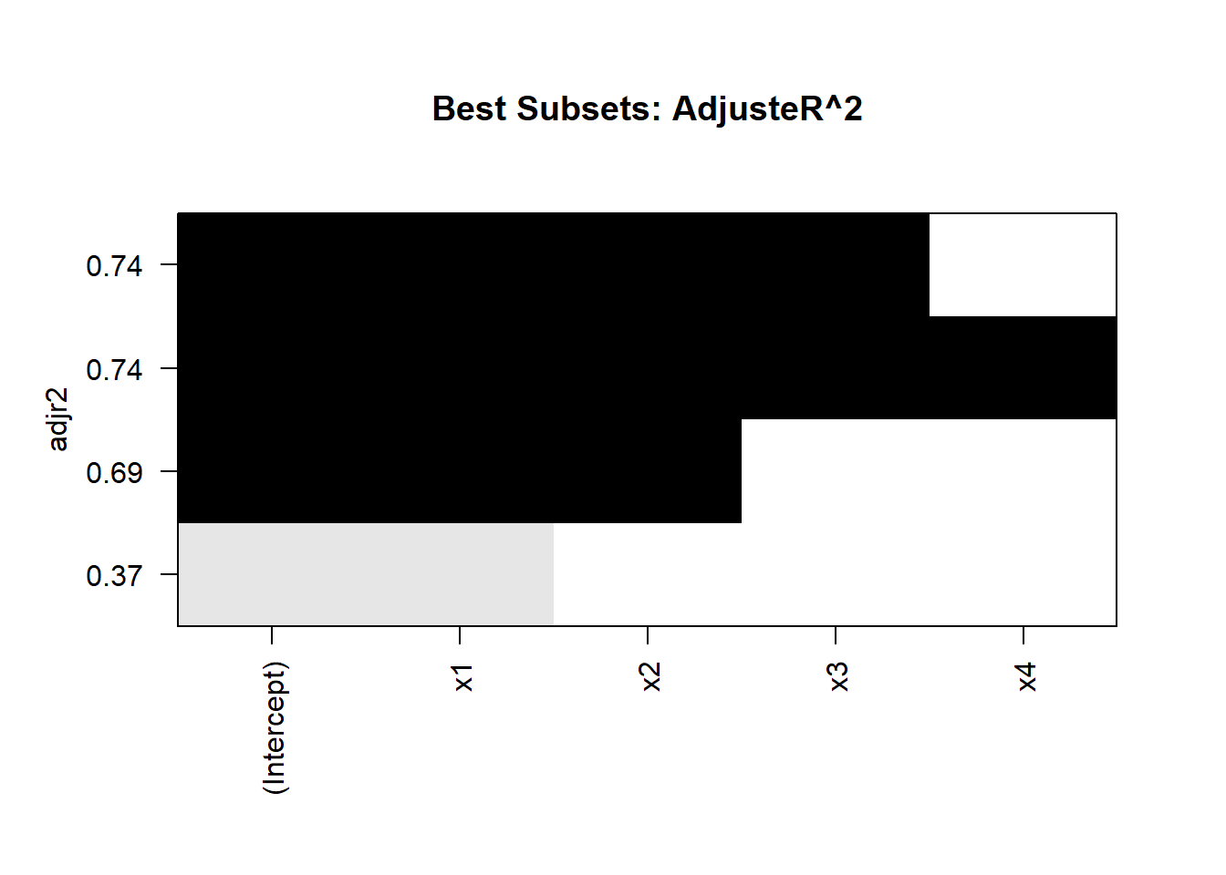
Figure 15.1: Best Subset Adjusted R2
Interpretation
Optimal Subsets:
The algorithm identifies the best subset of predictors for each model size.
Evaluate models based on metrics like adjusted \(R^2\), BIC, or AIC.
Visualization:
- The plot of adjusted \(R^2\) helps identify the model size with the best tradeoff between fit and complexity.
Efficiency:
- The Branch-and-Bound Algorithm achieves optimal results without evaluating all \(2^p\) subsets.
Advantages:
Guarantees the best subset for a given criterion.
Reduces computational cost compared to exhaustive search.
Handles moderate-sized problems efficiently.
Limitations:
Computationally intensive for very large datasets or many predictors (\(p > 20\)).
Requires a clearly defined evaluation criterion.
Practical Considerations
When to use Branch-and-Bound?
When \(p\) (number of predictors) is moderate (\(p \leq 20\)).
When global optimality for subset selection is essential.
Alternatives:
- For larger \(p\), consider heuristic methods like stepwise selection or regularization techniques (e.g., LASSO, Ridge).
Applications:
- Branch-and-Bound is widely used in fields like statistics, operations research, and machine learning where optimal subset selection is crucial.
15.2.4 Recursive Feature Elimination
Recursive Feature Elimination (RFE) is a feature selection method that systematically removes predictors from a model to identify the most relevant subset. RFE is commonly used in machine learning and regression tasks to improve model interpretability and performance by eliminating irrelevant or redundant features.
Theoretical Foundation
- Objective:
- Select the subset of predictors that maximizes the performance of the model (e.g., minimizes prediction error or maximizes explained variance).
- Approach:
- RFE is a backward selection method that recursively removes the least important predictors based on their contribution to the model’s performance.
- Key Features:
- Feature Ranking: Predictors are ranked based on their importance (e.g., weights in a linear model, coefficients in regression, or feature importance scores in tree-based models).
- Recursive Elimination: At each step, the least important predictor is removed, and the model is refit with the remaining predictors.
- Evaluation Criterion:
- Model performance is evaluated using metrics such as \(R^2\), AIC, BIC, or cross-validation scores.
Steps in RFE
- Initialize:
- Start with the full set of predictors.
- Rank Features:
- Train the model and compute feature importance scores (e.g., coefficients, weights, or feature importance).
- Eliminate Features:
- Remove the least important feature(s) based on the ranking.
- Refit Model:
- Refit the model with the reduced set of predictors.
- Repeat:
- Continue the process until the desired number of features is reached.
# Install and load caret package
if (!requireNamespace("caret", quietly = TRUE)) install.packages("caret")
library(caret)

# Simulated data
set.seed(123)
n <- 100
p <- 10
X <- matrix(rnorm(n * p), nrow = n, ncol = p)
y <- 5 + rowSums(X[, 1:3]) + rnorm(n, sd = 2)  # Only first 3 variables are relevant

# Convert to a data frame
data <- as.data.frame(X)
data$y <- y

# Define control for RFE
control <- rfeControl(functions = lmFuncs, # Use linear model for evaluation
                      method = "cv",      # Use cross-validation
                      number = 10)        # Number of folds

# Perform RFE
set.seed(123)
rfe_result <- rfe(data[, -ncol(data)], data$y,
                  sizes = c(1:10),          # Subset sizes to evaluate
                  rfeControl = control)

# Display RFE results
cat("Selected Predictors:\n")
#> Selected Predictors:
print(predictors(rfe_result))
#> [1] "V1" "V2" "V3"

cat("\nModel Performance:\n")
#>
#> Model Performance:
print(rfe_result$results)
#>    Variables     RMSE  Rsquared      MAE    RMSESD RsquaredSD     MAESD
#> 1          1 2.342391 0.2118951 1.840089 0.5798450  0.2043123 0.4254393
#> 2          2 2.146397 0.3549917 1.726721 0.5579553  0.2434206 0.4490311
#> 3          3 2.063923 0.4209751 1.662022 0.5362445  0.2425727 0.4217594
#> 4          4 2.124035 0.3574168 1.698954 0.5469199  0.2261644 0.4212677
#> 5          5 2.128605 0.3526426 1.684169 0.5375931  0.2469891 0.4163273
#> 6          6 2.153916 0.3226917 1.712140 0.5036119  0.2236060 0.4058412
#> 7          7 2.162787 0.3223240 1.716382 0.5089243  0.2347677 0.3940646
#> 8          8 2.152186 0.3222999 1.698816 0.5064040  0.2419215 0.3826101
#> 9          9 2.137741 0.3288444 1.687136 0.5016526  0.2436893 0.3684675
#> 10        10 2.139102 0.3290236 1.684362 0.5127830  0.2457675 0.3715176
Figure 15.2: RMSE CV
Interpretation
Selected Predictors:
- The algorithm identifies the most relevant predictors based on their impact on model performance.
Model Performance:
- The cross-validation results indicate how the model performs with different subset sizes, helping to select the optimal number of features.
Feature Ranking:
- RFE ranks features by their importance, providing insights into which predictors are most influential.
Advantages:
Improved Interpretability: Reduces the number of predictors, simplifying the model.
Performance Optimization: Eliminates irrelevant or redundant features, improving predictive accuracy.
Flexibility: Works with various model types (e.g., linear models, tree-based methods, SVMs).
Limitations:
Computationally Intensive: Repeatedly trains models, which can be slow for large datasets or complex models.
Model Dependency: Feature importance rankings depend on the underlying model, which may introduce bias.
Practical Considerations
When to use RFE?
For high-dimensional datasets where feature selection is critical for model interpretability and performance.
In machine learning workflows where feature importance scores are available.
Extensions:
Combine RFE with regularization methods (e.g., LASSO, Ridge) for additional feature selection.
Use advanced models (e.g., Random Forest, Gradient Boosting) for feature ranking.