30.13 Concerns in DID
30.13.1 Limitations and Common Issues
- Functional Form Dependence
- If the response to treatment is nonlinear, compare high- vs. low-intensity groups.
- Selection on (Time-Varying) Unobservables
- Use Rosenbaum Bounds to check the sensitivity of estimates to unobserved confounders.
- Long-Term Effects
- Parallel trends are more reliable in short time windows.
- Over long periods, other confounding factors may emerge.
- Heterogeneous Effects
- Treatment intensity (e.g., different doses) may vary across groups, leading to different effects.
- Ashenfelter’s Dip (Ashenfelter 1978)
- Participants in job training programs often experience earnings drops before enrolling, making them systematically different from nonparticipants.
- Fix: Compute long-run differences, excluding periods around treatment, to test for sustained impact (Proserpio and Zervas 2017; J. J. Heckman, LaLonde, and Smith 1999; Jepsen, Troske, and Coomes 2014).
- Lagged Treatment Effects
- If effects are not immediate, using a lagged dependent variable \(Y_{it-1}\) may be more appropriate (Blundell and Bond 1998).
- Bias from Unobserved Factors Affecting Trends
- If external shocks influence treatment and control groups differently, this biases DiD estimates.
- Correlated Observations
- Standard errors should be clustered appropriately.
- Incidental Parameters Problem (Lancaster 2000)
- Always prefer individual and time fixed effects to reduce bias.
- Treatment Timing and Negative Weights
- If treatment timing varies across units, negative weights can arise in standard DiD estimators when treatment effects are heterogeneous (Athey and Imbens 2022; Borusyak, Jaravel, and Spiess 2024; Goodman-Bacon 2021).
- Fix: Use estimators from Callaway and Sant’Anna (2021) and Clément De Chaisemartin and d’Haultfoeuille (2020) (
didpackage). - If expecting lags and leads, see L. Sun and Abraham (2021).
- Treatment Effect Heterogeneity Across Groups
- If treatment effects vary across groups and interact with treatment variance, standard estimators may be invalid (Gibbons, Suárez Serrato, and Urbancic 2018).
- Endogenous Timing
If the timing of units can be influenced by strategic decisions in a DID analysis, an instrumental variable approach with a control function can be used to control for endogeneity in timing.
- Questionable Counterfactuals
In situations where the control units may not serve as a reliable counterfactual for the treated units, matching methods such as propensity score matching or generalized random forest can be utilized. Additional methods can be found in Matching Methods.
30.13.2 Matching Methods in DID
Matching methods are often used in causal inference to balance treated and control units based on pre-treatment observables. In the context of Difference-in-Differences, matching helps:
- Reduce selection bias by ensuring that treated and control units are comparable before treatment.
- Improve parallel trends validity by selecting control units with similar pre-treatment trajectories.
- Enhance robustness when treatment assignment is non-random across groups.
Key Considerations in Matching
- Standard Errors Need Adjustment
- Standard errors should account for the fact that matching reduces variance (J. J. Heckman, Ichimura, and Todd 1997).
- A more robust alternative is Doubly Robust DID (Sant’Anna and Zhao 2020), where either matching or regression suffices for unbiased treatment effect identification.
- Group Fixed Effects Alone Do Not Eliminate Selection Bias
- Fixed effects absorb time-invariant heterogeneity, but do not correct for selection into treatment.
- Matching helps close the “backdoor path” between:
- Propensity to be treated
- Dynamics of outcome evolution post-treatment
- Matching on Time-Varying Covariates
- Beware of regression to the mean: extreme pre-treatment outcomes may artificially bias post-treatment estimates (Daw and Hatfield 2018).
- This issue is less concerning for time-invariant covariates.
- Comparing Matching vs. DID Performance
- Matching and DID both use pre-treatment outcomes to mitigate selection bias.
- Simulations (Chabé-Ferret 2015) show that:
- Matching tends to underestimate the true treatment effect but improves with more pre-treatment periods.
- When selection bias is symmetric, Symmetric DID (equal pre- and post-treatment periods) performs well.
- When selection bias is asymmetric, DID generally outperforms Matching.
- Forward DID as a Control Unit Selection Algorithm
- An efficient way to select control units is Forward DID (K. T. Li 2024).
30.13.3 Control Variables in DID
- Always report results with and without controls:
- If controls are fixed within groups or time periods, they should be absorbed in fixed effects.
- If controls vary across both groups and time, this suggests the parallel trends assumption is questionable.
- \(R^2\) is not crucial in causal inference:
- Unlike predictive models, causal models do not prioritize explanatory power (\(R^2\)), but rather unbiased identification of treatment effects.
30.13.4 DID for Count Data: Fixed-Effects Poisson Model
For count data, one can use the fixed-effects Poisson pseudo-maximum likelihood estimator (PPML) (Athey and Imbens 2006; Puhani 2012). Applications of this method can be found in management (Burtch, Carnahan, and Greenwood 2018) and marketing (C. He et al. 2021).
This approach offers robust standard errors under over-dispersion (Wooldridge 1999) and is particularly useful when dealing with excess zeros in the data.
Key advantages of PPML:
- Handles zero-inflated data better than log-OLS: A log-OLS regression may produce biased estimates (O’Hara and Kotze 2010) when heteroskedasticity is present (Silva and Tenreyro 2006), especially in datasets with many zeros (Silva and Tenreyro 2011).
- Avoids the limitations of negative binomial fixed effects: Unlike Poisson, there is no widely accepted fixed-effects estimator for the negative binomial model (Allison and Waterman 2002).
30.13.5 Handling Zero-Valued Outcomes in DID
When dealing with zero-valued outcomes, it is crucial to separate the intensive margin effect (e.g., outcome changes from 10 to 11) from the extensive margin effect (e.g., outcome changes from 0 to 1).
A common issue is that the treatment coefficient from a log-transformed regression cannot be directly interpreted as a percentage change when zeros are present (J. Chen and Roth 2024). To address this, we can consider two alternative approaches:
- Proportional Treatment Effects
We define the percentage change in the treated group’s post-treatment outcome as:
\[ \theta_{ATT\%} = \frac{E[Y_{it}(1) \mid D_i = 1, Post_t = 1] - E[Y_{it}(0) \mid D_i = 1, Post_t = 1]}{E[Y_{it}(0) \mid D_i = 1, Post_t = 1]} \]
Instead of assuming parallel trends in levels, we can rely on a parallel trends assumption in ratios (Wooldridge 2023).
The Poisson QMLE model is:
\[ Y_{it} = \exp(\beta_0 + \beta_1 D_i \times Post_t + \beta_2 D_i + \beta_3 Post_t + X_{it}) \epsilon_{it} \]
The treatment effect is estimated as:
\[ \hat{\theta}_{ATT\%} = \exp(\hat{\beta}_1) - 1 \]
To validate the parallel trends in ratios assumption, we can estimate a dynamic Poisson QMLE model:
\[ Y_{it} = \exp(\lambda_t + \beta_2 D_i + \sum_{r \neq -1} \beta_r D_i \times (RelativeTime_t = r)) \]
If the assumption holds, we expect:
\[ \exp(\hat{\beta}_r) - 1 = 0 \quad \text{for} \quad r < 0. \]
Even if the pre-treatment estimates appear close to zero, we should still conduct a sensitivity analysis (Rambachan and Roth 2023) to assess robustness (see Prior Parallel Trends Test).
set.seed(123) # For reproducibility

n <- 500 # Number of observations per group (treated and control)
# Generating IDs for a panel setup
ID <- rep(1:n, times = 2)

# Defining groups and periods
Group     <- rep(c("Control", "Treated"), each = n)
Time      <- rep(c("Before", "After"), times = n)
Treatment <- ifelse(Group == "Treated", 1, 0)
Post      <- ifelse(Time == "After", 1, 0)

# Step 1: Generate baseline outcomes with a zero-inflated model
lambda <- 20 # Average rate of occurrence
zero_inflation <- 0.5 # Proportion of zeros
Y_baseline <-
    ifelse(runif(2 * n) < zero_inflation, 0, rpois(2 * n, lambda))

# Step 2: Apply DiD treatment effect on the treated group in the post-treatment period
Treatment_Effect <- Treatment * Post
Y_treatment <-
    ifelse(Treatment_Effect == 1, rpois(n, lambda = 2), 0)

# Incorporating a simple time trend, ensuring outcomes are non-negative
Time_Trend <- ifelse(Time == "After", rpois(2 * n, lambda = 1), 0)

# Step 3: Combine to get the observed outcomes
Y_observed <- Y_baseline + Y_treatment + Time_Trend

# Ensure no negative outcomes after the time trend
Y_observed <- ifelse(Y_observed < 0, 0, Y_observed)

# Create the final dataset
data <-
    data.frame(
        ID = ID,
        Treatment = Treatment,
        Period = Post,
        Outcome = Y_observed
    )

# Viewing the first few rows of the dataset
head(data)
#>   ID Treatment Period Outcome
#> 1  1         0      0       0
#> 2  2         0      1      25
#> 3  3         0      0       0
#> 4  4         0      1      20
#> 5  5         0      0      19
#> 6 6 0 1 0library(fixest)
res_pois <-
fepois(Outcome ~ Treatment + Period + Treatment * Period,
data = data,
vcov = "hetero")
etable(res_pois)
#> res_pois
#> Dependent Var.: Outcome
#>
#> Constant 2.249*** (0.0717)
#> Treatment 0.1743. (0.0932)
#> Period 0.0662 (0.0960)
#> Treatment x Period 0.0314 (0.1249)
#> __________________ _________________
#> S.E. type Heteroskeda.-rob.
#> Observations 1,000
#> Squared Cor. 0.01148
#> Pseudo R2 0.00746
#> BIC 15,636.8
#> ---
#> Signif. codes: 0 '***' 0.001 '**' 0.01 '*' 0.05 '.' 0.1 ' ' 1
# Average percentage change
exp(coefficients(res_pois)["Treatment:Period"]) - 1
#> Treatment:Period
#> 0.03191643
# SE using delta method
exp(coefficients(res_pois)["Treatment:Period"]) *
sqrt(res_pois$cov.scaled["Treatment:Period", "Treatment:Period"])
#> Treatment:Period
#> 0.1288596In this example, the DID coefficient is not significant. However, say that it’s significant, we can interpret the coefficient as 3 percent increase in post-treatment period due to the treatment.
library(fixest)

base_did_log0 <- base_did |>
    mutate(y = if_else(y > 0, y, 0))

res_pois_es <-
    fepois(y ~ x1 + i(period, treat, 5) | id + period,
           data = base_did_log0,
           vcov = "hetero")

etable(res_pois_es)
#>                            res_pois_es
#> Dependent Var.:                      y
#>
#> x1                  0.1895*** (0.0108)
#> treat x period = 1    -0.2769 (0.3545)
#> treat x period = 2    -0.2699 (0.3533)
#> treat x period = 3     0.1737 (0.3520)
#> treat x period = 4    -0.2381 (0.3249)
#> treat x period = 6     0.3724 (0.3086)
#> treat x period = 7    0.7739* (0.3117)
#> treat x period = 8    0.5028. (0.2962)
#> treat x period = 9   0.9746** (0.3092)
#> treat x period = 10  1.310*** (0.3193)
#> Fixed-Effects:      ------------------
#> id                                 Yes
#> period                             Yes
#> ___________________ __________________
#> S.E. type           Heteroskedas.-rob.
#> Observations                     1,080
#> Squared Cor.                   0.51131
#> Pseudo R2                      0.34836
#> BIC                            5,868.8
#> ---
#> Signif. codes: 0 '***' 0.001 '**' 0.01 '*' 0.05 '.' 0.1 ' ' 1
Figure 30.27 shows the parallel trends before treatment and the effect after treatment.
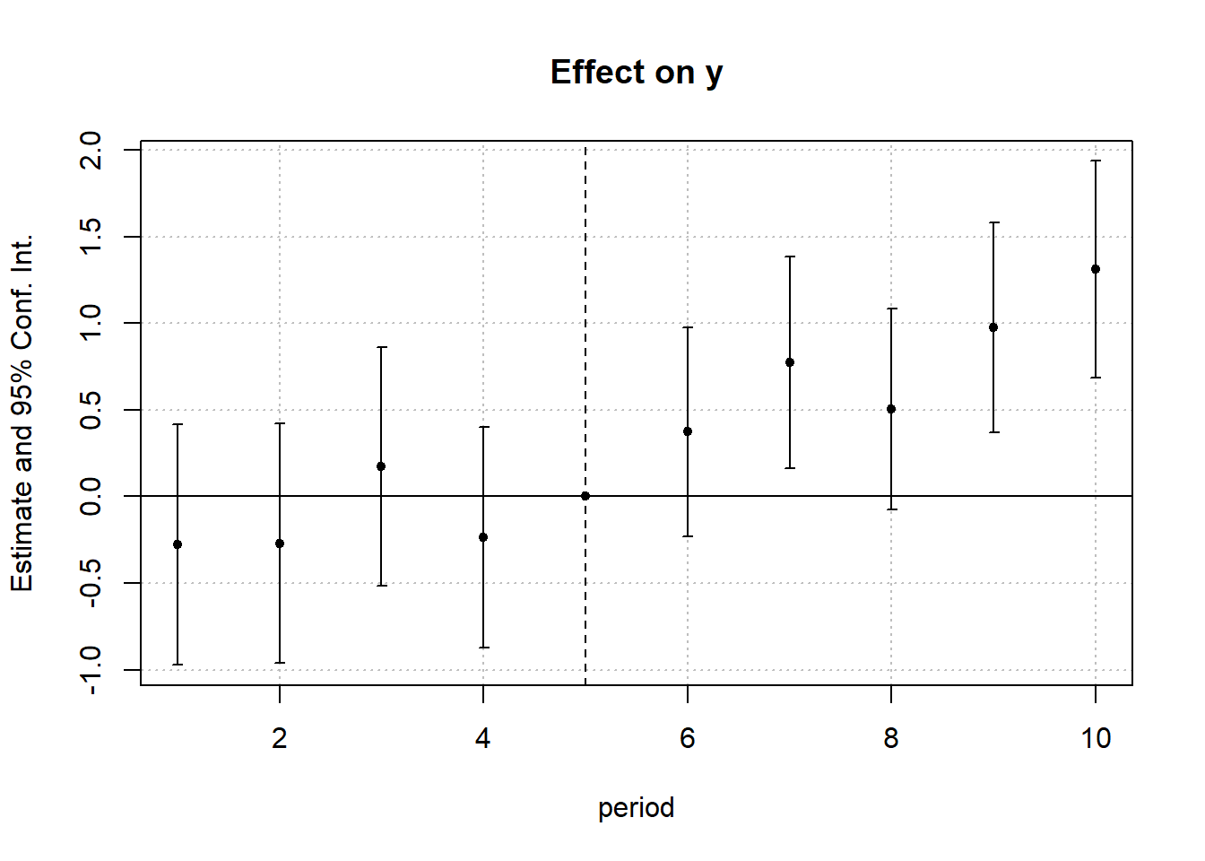
Figure 30.27: Event study estimates from Poisson regression model
This parallel trend is the “ratio” version as in Wooldridge (2023) :
\[ \frac{E(Y_{it}(0) |D_i = 1, Post_t = 1)}{E(Y_{it}(0) |D_i = 1, Post_t = 0)} = \frac{E(Y_{it}(0) |D_i = 0, Post_t = 1)}{E(Y_{it}(0) |D_i =0, Post_t = 0)} \]
which means without treatment, the average percentage change in the mean outcome for treated group is identical to that of the control group.
- Log Effects with Calibrated Extensive-Margin Value
A potential limitation of proportional treatment effects is that they may not be well-suited for heavy-tailed outcomes. In such cases, we may prefer to explicitly model the extensive margin effect.
Following (J. Chen and Roth 2024, 39), we can calibrate the weight placed on the intensive vs. extensive margin to ensure meaningful interpretation of the treatment effect.
If we want to study the treatment effect on a concave transformation of the outcome that is less influenced by those in the distribution’s tail, then we can perform this analysis.
Steps:
- Normalize the outcomes such that 1 represents the minimum non-zero and positive value (i.e., divide the outcome by its minimum non-zero and positive value).
- Estimate the treatment effects for the new outcome
\[ m(y) = \begin{cases} \log(y) & \text{for } y >0 \\ -x & \text{for } y = 0 \end{cases} \]
The choice of \(x\) depends on what the researcher is interested in:
| Value of \(x\) | Interest |
|---|---|
| \(x = 0\) | The treatment effect in logs where all zero-valued outcomes are set to equal the minimum non-zero value (i.e., we exclude the extensive-margin change between 0 and \(y_{min}\) ) |
| \(x>0\) | Setting the change between 0 and \(y_{min}\) to be valued as the equivalent of a \(x\) log point change along the intensive margin. |
library(fixest)
base_did_log0_cali <- base_did_log0 |>
    # get min
    mutate(min_y = min(y[y > 0])) |>

    # normalized the outcome
    mutate(y_norm = y / min_y)

my_regression <-
    function(x) {
        base_did_log0_cali <-
            base_did_log0_cali %>% mutate(my = ifelse(y_norm == 0,-x,
                                                      log(y_norm)))
        my_reg <-
            feols(
                fml = my ~ x1 + i(period, treat, 5) | id + period,
                data = base_did_log0_cali,
                vcov = "hetero"
            )

        return(my_reg)
    }

xvec <- c(0, .1, .5, 1, 3)
reg_list <- purrr::map(.x = xvec, .f = my_regression)


iplot(reg_list,
      pt.col =  1:length(xvec),
      pt.pch = 1:length(xvec))
legend("topleft",
       col = 1:length(xvec),
       pch = 1:length(xvec),
       legend = as.character(xvec))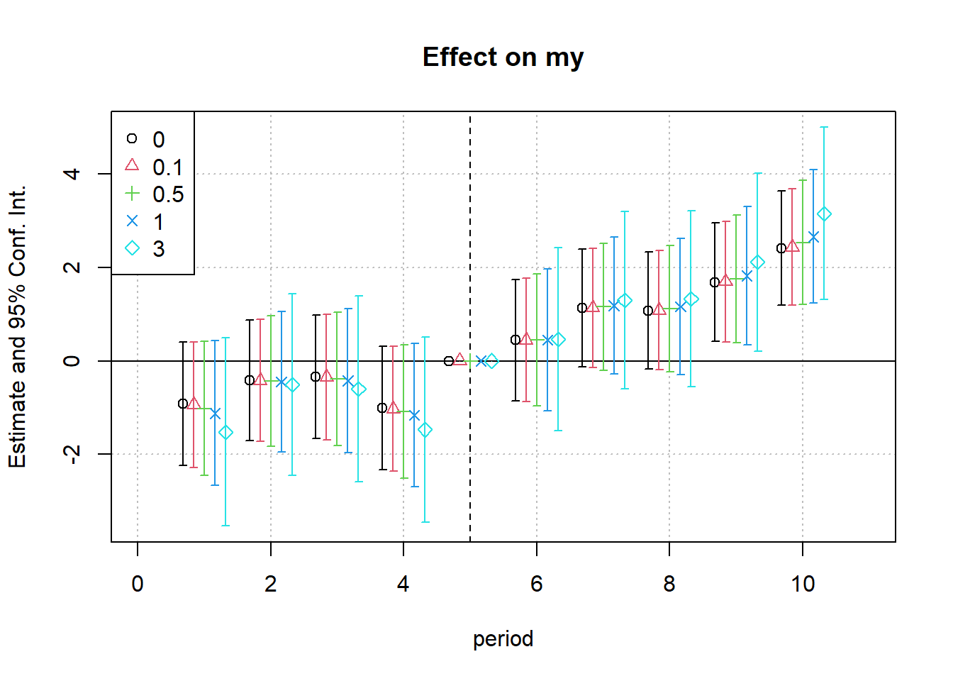
etable(
    reg_list,
    headers = list("Extensive-margin value (x)" = as.character(xvec)),
    digits = 2,
    digits.stats = 2
)
#>                                   model 1        model 2        model 3
#> Extensive-margin value (x)              0            0.1            0.5
#> Dependent Var.:                        my             my             my
#>
#> x1                         0.43*** (0.02) 0.44*** (0.02) 0.46*** (0.03)
#> treat x period = 1           -0.92 (0.67)   -0.94 (0.69)    -1.0 (0.73)
#> treat x period = 2           -0.41 (0.66)   -0.42 (0.67)   -0.43 (0.71)
#> treat x period = 3           -0.34 (0.67)   -0.35 (0.68)   -0.38 (0.73)
#> treat x period = 4            -1.0 (0.67)    -1.0 (0.68)    -1.1 (0.73)
#> treat x period = 6            0.44 (0.66)    0.44 (0.67)    0.45 (0.72)
#> treat x period = 7            1.1. (0.64)    1.1. (0.65)    1.2. (0.70)
#> treat x period = 8            1.1. (0.64)    1.1. (0.65)     1.1 (0.69)
#> treat x period = 9           1.7** (0.65)   1.7** (0.66)    1.8* (0.70)
#> treat x period = 10         2.4*** (0.62)  2.4*** (0.63)  2.5*** (0.68)
#> Fixed-Effects:             -------------- -------------- --------------
#> id                                    Yes            Yes            Yes
#> period                                Yes            Yes            Yes
#> __________________________ ______________ ______________ ______________
#> S.E. type                  Heterosk.-rob. Heterosk.-rob. Heterosk.-rob.
#> Observations                        1,080          1,080          1,080
#> R2                                   0.43           0.43           0.43
#> Within R2                            0.26           0.26           0.25
#>
#>                                   model 4        model 5
#> Extensive-margin value (x)              1              3
#> Dependent Var.:                        my             my
#>
#> x1                         0.49*** (0.03) 0.62*** (0.04)
#> treat x period = 1            -1.1 (0.79)     -1.5 (1.0)
#> treat x period = 2           -0.44 (0.77)   -0.51 (0.99)
#> treat x period = 3           -0.43 (0.78)    -0.60 (1.0)
#> treat x period = 4            -1.2 (0.78)     -1.5 (1.0)
#> treat x period = 6            0.45 (0.77)     0.46 (1.0)
#> treat x period = 7             1.2 (0.75)     1.3 (0.97)
#> treat x period = 8             1.2 (0.74)     1.3 (0.96)
#> treat x period = 9            1.8* (0.75)    2.1* (0.97)
#> treat x period = 10         2.7*** (0.73)  3.2*** (0.94)
#> Fixed-Effects:             -------------- --------------
#> id                                    Yes            Yes
#> period                                Yes            Yes
#> __________________________ ______________ ______________
#> S.E. type                  Heterosk.-rob. Heterosk.-rob.
#> Observations                        1,080          1,080
#> R2                                   0.42           0.41
#> Within R2                            0.25           0.24
#> ---
#> Signif. codes: 0 '***' 0.001 '**' 0.01 '*' 0.05 '.' 0.1 ' ' 1
We have the dynamic treatment effects for different hypothesized extensive-margin value of \(x \in (0, .1, .5, 1, 3, 5)\)
The first column is when the zero-valued outcome equal to \(y_{min, y>0}\) (i.e., there is no different between the minimum outcome and zero outcome - \(x = 0\))
For this particular example, as the extensive margin increases, we see an increase in the effect magnitude. The second column is when we assume an extensive-margin change from 0 to \(y_{min, y >0}\) is equivalent to a 10 (i.e., \(0.1 \times 100\)) log point change along the intensive margin.
30.13.6 Standard Errors
One of the major statistical challenges in DiD estimation is serial correlation in the error terms. This issue is particularly problematic because it can lead to underestimated standard errors, inflating the likelihood of Type I errors (false positives). As discussed in Bertrand, Duflo, and Mullainathan (2004), serial correlation arises in DiD settings due to several factors:
- Long time series: Many DiD studies use multiple time periods, increasing the risk of correlated errors.
- Highly positively serially correlated outcomes: Many economic and business variables (e.g., GDP, sales, employment rates) exhibit strong persistence over time.
- Minimal within-group variation in treatment timing: For example, in a state-level policy change, all individuals in a state receive treatment at the same time, leading to correlation within state-time clusters.
To correct for serial correlation, various methods can be employed. However, some approaches work better than others:
- Avoid standard parametric corrections: A common approach is to model the error term using an autoregressive (AR) process. However, Bertrand, Duflo, and Mullainathan (2004) show that this often fails in DiD settings because it does not fully account for within-group correlation.
- Nonparametric solutions (preferred when the number of groups is large):
- Block bootstrap: Resampling entire groups (e.g., states) rather than individual observations maintains the correlation structure and provides robust standard errors.
- Collapsing data into two periods (Pre vs. Post):
- Aggregating the data into a single pre-treatment and single post-treatment period can mitigate serial correlation issues. This approach is particularly useful when the number of groups is small (Donald and Lang 2007).
- Note: While this reduces the power of the analysis by discarding variation across time, it ensures that standard errors are not artificially deflated.
- Variance-covariance matrix corrections:
- Empirical corrections (e.g., cluster-robust standard errors) and arbitrary variance-covariance matrix adjustments (e.g., Newey-West) can work well, but they are reliable only in large samples.
Overall, selecting the appropriate correction method depends on the sample size and structure of the data. When possible, block bootstrapping and collapsing data into pre/post periods are among the most effective approaches.
30.13.7 Partial Identification
Classical DiD delivers a point‑identified estimate of the average treatment effect on the treated (ATT) only when the parallel‑trends assumption is exact. Yet in practice pre‑trends often deviate or post‑treatment shocks differ across groups (e.g., the famous Ashenfelter (1978)). Partial‑identification (PI) methods shift the question from “Is the estimate unbiased?” to “How much would the identifying assumption have to fail before I reverse my conclusion?”
PI approaches for DiD
- Manski and Pepper (2018) propose bounding the treatment effect parameter \(\delta\) across time and space in the presence of violations to the parallel trends assumption.
- L. J. Keele et al. (2019) introduce a Rosenbaum-style sensitivity parameter that quantifies the magnitude of hidden bias necessary to reverse the sign of the estimated effect.
- L. Keele, Hasegawa, and Small (2019) extends this framework to settings where the treated group may be simultaneously exposed to another event, using the Rosenbaum-style sensitivity analysis to assess the robustness of causal claims under such compound treatments.
- Ye et al. (2024) utilize two control groups subjected to negatively correlated shocks to non-parametrically bracket the counterfactual trend, offering bounds on treatment effects without relying on the parallel trends assumption.
- Leavitt (2020) adopts an Empirical Bayes approach that places a hierarchical prior over \(\delta\), shrinking extreme violations of parallel trends while providing posterior credible intervals that explicitly account for trend heterogeneity.
- Two bounding strategies in Rambachan and Roth (2023)
- Relative magnitude bounds: \(|\delta| \leq M \cdot \max\) pre-period jumps
- Smoothness bounds: allow \(\delta\)’s slope to shift by at most \(M\) per period.
30.13.7.1 Canonical DiD notation and the source of bias
Let
- \(Y_{it}^{1}\) and \(Y_{it}^{0}\) be potential outcomes for unit \(i\) in period \(t\) under treatment and no treatment;
- \(D_i\in\{0,1\}\) indicate ever‑treated units;
- \(\texttt{Post}_t\) mark periods after the policy shock.
For two periods (pre, post) and two groups (T = treated, U = untreated) the simple DiD estimator is
\[ \hat\beta_{DD}= \left[E(Y_T^{1}\mid \texttt{Post})-E(Y_T^{0}\mid \texttt{Pre})\right]-\left[E(Y_U^{0}\mid \texttt{Post})-E(Y_U^{0}\mid \texttt{Pre})\right] \]
Add and subtract the counterfactual trend \(E(Y_T^{0}\mid \texttt{Post})\) and rearrange:
\[ \begin{aligned} \hat\beta_{DD} &= \underbrace{E(Y_T^{1}\mid\texttt{Post})-E(Y_T^{0}\mid\texttt{Post})}_{\text{ATT}} \\ &+ \underbrace{\bigl[E(Y_T^{0}\mid\texttt{Post})-E(Y_T^{0}\mid\texttt{Pre})\bigr] -\bigl[E(Y_U^{0}\mid\texttt{Post})-E(Y_U^{0}\mid\texttt{Pre})\bigr]}_{\delta} \end{aligned} \]
Hence
\[ \hat\beta_{DD}= \text{ATT}+\delta . \]
When parallel trends hold, \(\delta=0\); any violation translates one‑for‑one into bias (Frake et al. 2025).
30.13.7.2 Bounding the ATT when \(\delta\neq 0\)
The core PI idea is simple: derive credible bounds on \(\delta\), then translate those into bounds on the ATT.
Two families of restrictions, both operationalized by Rambachan and Roth (2023) and implemented in the honestdid package, are now widely used:
- Relative‑magnitude (RM) bounds: the post‑treatment gap \(|\delta|\) cannot exceed \(M\) times the largest period‑to‑period deviation observed in the pre‑treatment event‑study.
- Smoothness (SM) bounds: the slope of the treated‑minus‑control gap can change by at most \(M\) units each period after treatment.
Because \(M\) is researcher‑chosen, inference is reported across a grid of plausible \(M\) values, revealing the breakdown threshold where the confidence set first touches zero (Frake et al. 2025, 14).
30.13.7.3 Relative‑Magnitude Restriction {#sec-relative‑magnitude-restriction-honestdid}}
Let \(\hat g_t\) be the event‑study coefficient at time \(t\) (normalized to zero at \(t=-1\)).
Step 1: calibrate the worst pre‑trend:
\(M_0 = \max_{s<0} |\hat g_s-\hat g_{s-1}|\).Step 2: allow proportional violations post‑treatment:
Impose \(|\delta_t|\le M\cdot M_0\) for every \(t\ge 0\).Step 3: construct “honest” confidence sets for the ATT or for period‑specific effects by solving a constrained least‑squares problem (Rambachan and Roth 2023).
30.13.7.4 Smoothness Restriction
When violations evolve gradually (e.g., treated units drift upward over time), the SM bound is more credible.
Step 1: estimate the pre‑treatment slope:
\(s_0 = \hat g_{-1}-\hat g_{-2}\).Step 2: restrict post‑treatment slopes:
The counterfactual slope in period \(k\) may vary within
\([s_0-M, s_0+M]\).Step 3: propagate forward to obtain an admissible path for \(\delta_t\); compute the least‑favorable path, then derive confidence sets (Rambachan and Roth 2023).
30.13.7.5 Step‑by‑step Empirical Workflow
See Frake et al. (2025), p. 15 for a decision tree that guides the choice of method.
- Graph the event‑study. Are any pre‑trends visible? Quantify their magnitude and/or slope.
- Choose a restriction family (RM for episodic shocks, SM for trending deviations). Justify the choice theoretically (e.g., anticipation effects vs. gradual selection).
- Select a grid of \(M\). Always display the break‑even \(M^{*}\) where the CI first covers zero; interpret \(M^{*}\) in real‑world units.
- Report the full set, not only the “robust” interval. Transparency trumps opportunistic suppression.
- Complement with falsification tests (placebo policy dates, placebo outcomes) to discipline the plausible range of \(M\).
- Document software and code.
honestdid(R/Stata) includes convenient wrappers for both restrictions and automatic figures.
30.13.7.6 Worked Example (Stylized)
Suppose pre‑policy trends exhibit at most a 0.8‑point swing. Setting \(M\in\{0,0.5,1,1.5\}\):
| \(M\) | 95 % CI for ATT | Conclusion |
|---|---|---|
| 0 | [0.85, 1.25] | Positive, robust |
| 0.5 | [0.60, 1.50] | Positive |
| 1 | [‑0.05, 1.85] | Sign flips plausible |
| 1.5 | [‑0.45, 2.25] | Cannot rule out zero |
Thus the causal claim survives unless the unobserved counterfactual deviations are \(\ge 1 \times\) the worst pre‑treatment kink, an interpretation far clearer than a single \(p\)‑value.
30.13.7.7 Common Pitfalls and Best Practices
- Mistaking absence of significant pre‑trends for proof of parallel‑trends. Under‑powered tests can miss economically large differences.
- Choosing \(M\) post‑hoc. Decide the grid before looking at results.
- Ignoring sign. If theory predicts the treated counterfactual would have fallen, impose a one‑sided bound; doing otherwise wastes power.
- Forgetting heterogeneous timing or staggered adoption. Apply PI to group‑time ATT estimates from modern DiD estimators before aggregation.
Partial‑identification transforms DiD from a “take‑it‑or‑leave‑it” enterprise into a transparent sensitivity analysis. By explicitly parameterizing and visually communicating, the extent of permissible departures from parallel trends, researchers allow readers to map their own priors onto empirical conclusions. Used thoughtfully, PI techniques enhance credibility without demanding the impossible.