3.3 Normality Assessment
The Normal (Gaussian) distribution plays a critical role in statistical analyses due to its theoretical and practical applications. Many statistical methods assume normality in the data, making it essential to assess whether our variable of interest follows a normal distribution. To achieve this, we utilize both Numerical Measures and Graphical Assessment.
3.3.1 Graphical Assessment
Graphical methods provide an intuitive way to visually inspect the normality of a dataset. One of the most common methods is the Q-Q plot (quantile-quantile plot). The Q-Q plot compares the quantiles of the sample data to the quantiles of a theoretical normal distribution. Deviations from the line indicate departures from normality.
Below is an example of using the qqnorm and qqline functions in R to assess the normality of the precip dataset, which contains precipitation data (in inches per year) for 70 U.S. cities:
# Load the required package
pacman::p_load("car")

# Generate a Q-Q plot
qqnorm(precip,
       ylab = "Precipitation [in/yr] for 70 US cities",
       main = "Q-Q Plot of Precipitation Data")
qqline(precip, col = "red")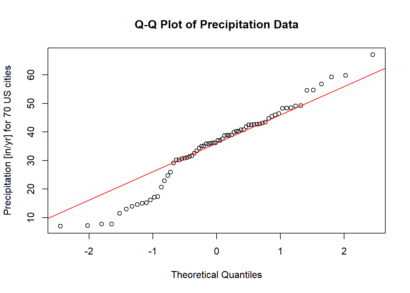
Figure 2.12: Q-Q Plot of Precipitation Data
Interpretation
Theoretical Line: The red line represents the expected relationship if the data were perfectly normally distributed.
Data Points: The dots represent the actual empirical data.
If the points closely align with the theoretical line, we can conclude that the data likely follow a normal distribution. However, noticeable deviations from the line, particularly systematic patterns (e.g., curves or s-shaped patterns), indicate potential departures from normality.
Tips
Small Deviations: Minor deviations from the line in small datasets are not uncommon and may not significantly impact analyses that assume normality.
Systematic Patterns: Look for clear trends, such as clusters or s-shaped curves, which suggest skewness or heavy tails.
Complementary Tests: Always pair graphical methods with numerical measures (e.g., Shapiro-Wilk test) to make a robust conclusion.
When interpreting a Q-Q plot, it is helpful to see both ideal and non-ideal scenarios. Below is an illustrative example:
Normal Data: Points fall closely along the line.
Skewed Data: Points systematically deviate from the line, curving upward or downward.
Heavy Tails: Points deviate at the extremes (ends) of the distribution.
By combining visual inspection and numerical measures, we can better understand the nature of our data and its alignment with the assumption of normality.
3.3.2 Summary Statistics
While graphical assessments, such as Q-Q plots, provide a visual indication of normality, they may not always offer a definitive conclusion. To supplement graphical methods, statistical tests are often employed. These tests provide quantitative evidence to support or refute the assumption of normality. The most common methods can be classified into two categories:
3.3.2.1 Methods Based on Normal Probability Plot
3.3.2.1.1 Correlation Coefficient with Normal Probability Plots
As described by Looney and Gulledge Jr (1985) and Samuel S. Shapiro and Francia (1972), this method evaluates the linearity of a normal probability plot by calculating the correlation coefficient between the ordered sample values \(y_{(i)}\) and their theoretical normal quantiles \(m_i^*\). A perfectly linear relationship suggests that the data follow a normal distribution.
The correlation coefficient, denoted \(W^*\), is given by:
\[ W^* = \frac{\sum_{i=1}^{n}(y_{(i)}-\bar{y})(m_i^* - 0)}{\sqrt{\sum_{i=1}^{n}(y_{(i)}-\bar{y})^2 \cdot \sum_{i=1}^{n}(m_i^* - 0)^2}} \]
where:
\(\bar{y}\) is the sample mean,
\(\bar{m^*} = 0\) under the null hypothesis of normality.
The Pearson product-moment correlation formula can also be used to evaluate this relationship:
\[ \hat{\rho} = \frac{\sum_{i=1}^{n}(y_i - \bar{y})(x_i - \bar{x})}{\sqrt{\sum_{i=1}^{n}(y_i - \bar{y})^2 \cdot \sum_{i=1}^{n}(x_i - \bar{x})^2}} \]
- Interpretation:
- When the correlation is 1, the plot is exactly linear, and normality is assumed.
- The closer the correlation is to 0, the stronger the evidence to reject normality.
- Inference on \(W^*\) requires reference to special tables (Looney and Gulledge Jr 1985).
3.3.2.1.2 Shapiro-Wilk Test
The Shapiro-Wilk test (Samuel Sanford Shapiro and Wilk 1965) is one of the most widely used tests for assessing normality, especially for sample sizes \(n < 2000\). This test evaluates how well the data’s order statistics match a theoretical normal distribution. The test statistic, \(W\), is computed as:
\[ W=\frac{\sum_{i=1}^{n}a_i x_{(i)}}{\sum_{i=1}^{n}(x_{(i)}-\bar{x})^2} \]
where
\(n\): The sample size.
\(x_{(i)}\): The \(i\)-th smallest value in the sample (the ordered data).
\(\bar{x}\): The sample mean.
\(a_i\): Weights derived from the expected values and variances of the order statistics of a normal distribution, precomputed based on the sample size \(n\).
Sensitive to:
- Symmetry
- The Shapiro-Wilk test assesses whether a sample is drawn from a normal distribution, which assumes symmetry around the mean.
- If the data exhibit skewness (a lack of symmetry), the test is likely to reject the null hypothesis of normality.
- Heavy Tails
- Heavy tails refer to distributions where extreme values (outliers) are more likely compared to a normal distribution.
- The Shapiro-Wilk test is also sensitive to such departures from normality because heavy tails affect the spread and variance, which are central to the calculation of the test statistic \(W\).
Hence, the Shapiro-Wilk test’s sensitivity to these deviations makes it a powerful tool for detecting non-normality only in small to moderate-sized samples. However:
It is generally more sensitive to symmetry (skewness) than to tail behavior (kurtosis).
In very large samples, even small deviations in symmetry or tail behavior may cause the test to reject the null hypothesis, even if the data is practically “normal” for the intended analysis.
Small sample sizes may lack power to detect deviations from normality.
Large sample sizes may detect minor deviations that are not practically significant.
Key Steps:
Sort the Data: Arrange the sample data in ascending order, yielding \(x_{(1)}, x_{(2)}, \dots, x_{(n)}\).
Compute Weights: The weights \(a_i\) are determined using a covariance matrix of the normal order statistics. These are optimized to maximize the power of the test.
Calculate \(W\): Use the formula to determine \(W\), which ranges from 0 to 1.
Decision Rule:
Null Hypothesis (\(H_0\)): The data follows a normal distribution.
Alternative Hypothesis (\(H_1\)): The data does not follow a normal distribution.
A small \(W\) value, along with a \(p\)-value below a chosen significance level (e.g., 0.05), leads to rejection of \(H_0\).
Under normality, \(W\) approaches 1.
Smaller values of \(W\) indicate deviations from normality.
# Perform Shapiro-Wilk Test (Default for gofTest)
EnvStats::gofTest(mtcars$mpg, test = "sw")
#> $distribution
#> [1] "Normal"
#>
#> $dist.abb
#> [1] "norm"
#>
#> $distribution.parameters
#>      mean        sd
#> 20.090625  6.026948
#>
#> $n.param.est
#> [1] 2
#>
#> $estimation.method
#> [1] "mvue"
#>
#> $statistic
#>         W
#> 0.9475647
#>
#> $sample.size
#> [1] 32
#>
#> $parameters
#>  n
#> 32
#>
#> $z.value
#> [1] 1.160703
#>
#> $p.value
#> [1] 0.1228814
#>
#> $alternative
#> [1] "True cdf does not equal the\n                                 Normal Distribution."
#>
#> $method
#> [1] "Shapiro-Wilk GOF"
#>
#> $data
#>  [1] 21.0 21.0 22.8 21.4 18.7 18.1 14.3 24.4 22.8 19.2 17.8 16.4 17.3 15.2 10.4
#> [16] 10.4 14.7 32.4 30.4 33.9 21.5 15.5 15.2 13.3 19.2 27.3 26.0 30.4 15.8 19.7
#> [31] 15.0 21.4
#>
#> $data.name
#> [1] "mtcars$mpg"
#>
#> $bad.obs
#> [1] 0
#>
#> attr(,"class")
#> [1] "gof"
3.3.2.2 Methods Based on Empirical Cumulative Distribution Function
The Empirical Cumulative Distribution Function (ECDF) is a way to represent the distribution of a sample dataset in cumulative terms. It answers the question:
“What fraction of the observations in my dataset are less than or equal to a given value \(x\)?”
The ECDF is defined as:
\[ F_n(x) = \frac{1}{n} \sum_{i=1}^{n} \mathbb{I}(X_i \leq x) \]
where:
\(F_(x)\): ECDF at value \(x\).
\(n\): Total number of data points.
\(\mathbb{I}(X_i \leq x)\): Indicator function, equal to 1 if \(X_i \leq x\), otherwise 0.
This method is especially useful for large sample sizes and can be applied to distributions beyond the normal (Gaussian) distribution.
Properties of the ECDF
- Step Function: The ECDF is a step function that increases by \(1/n\) at each data point.
- Non-decreasing: As \(x\) increases, \(F_n(x)\) never decreases.
- Range: The ECDF starts at 0 and ends at 1:
- \(F_n(x) = 0\) for \(x < \min(X)\).
- \(F_n(x) = 1\) for \(x \geq \max(X)\).
- Convergence: As \(n \to \infty\), the ECDF approaches the true cumulative distribution function (CDF) of the population.
Let’s consider a sample dataset \(\{3, 7, 7, 10, 15\}\). The ECDF at different values of \(x\) is calculated as:
| \(x\) | \(\mathbb{I}(X_i \leq x)\) for each \(X_i\) | Count \(\leq x\) | ECDF \(F_n(x)\) |
|---|---|---|---|
| \(x = 5\) | \(\{1, 0, 0, 0, 0\}\) | 1 | \(1/5 = 0.2\) |
| \(x = 7\) | \(\{1, 1, 1, 0, 0\}\) | 3 | \(3/5 = 0.6\) |
| \(x = 12\) | \(\{1, 1, 1, 1, 0\}\) | 4 | \(4/5 = 0.8\) |
| \(x = 15\) | \(\{1, 1, 1, 1, 1\}\) | 5 | \(5/5 = 1.0\) |
Applications of the ECDF
Goodness-of-fit Tests: Compare the ECDF to a theoretical CDF (e.g., using the Kolmogorov-Smirnov test).
Outlier Detection: Analyze cumulative trends to spot unusual data points.
Visual Data Exploration: Use the ECDF to understand the spread, skewness, and distribution of the data.
Comparing Distributions: Compare the ECDFs of two datasets to assess differences in their distributions.
# Load required libraries
library(ggplot2)

# Sample dataset
data <- c(3, 7, 7, 10, 15)

# ECDF calculation
ecdf_function <- ecdf(data)

# Generate a data frame for plotting
ecdf_data <- data.frame(x = sort(unique(data)),
                        ecdf = sapply(sort(unique(data)), function(x)
                          mean(data <= x)))

# Display ECDF values
print(ecdf_data)
#>    x ecdf
#> 1  3  0.2
#> 2  7  0.6
#> 3 10  0.8
#> 4 15  1.0
# Plot the ECDF
ggplot(ecdf_data, aes(x = x, y = ecdf)) +
geom_step() +
labs(
title = "Empirical Cumulative Distribution Function",
x = "Data Values",
y = "Cumulative Proportion"
) +
theme_minimal()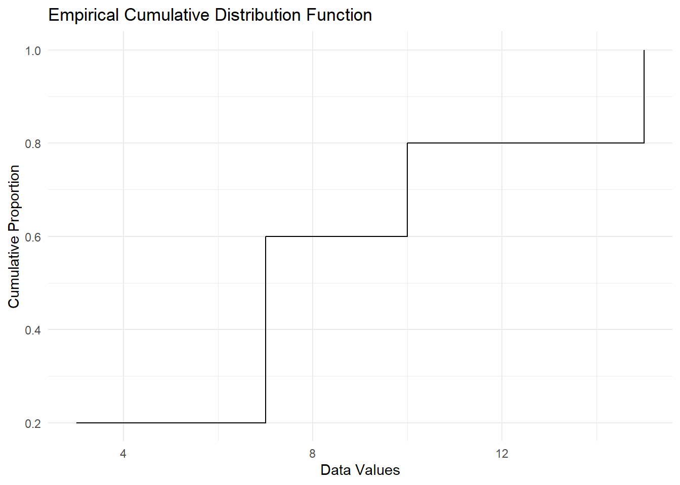
Figure 2.16: Empirical Cumulative Distribution Function
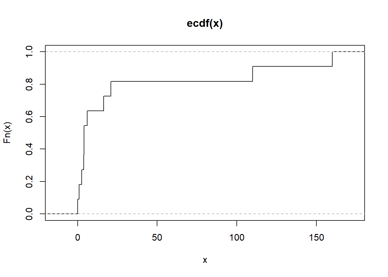
Figure 2.17: Empirical Cumulative Distribution Function Alternative
3.3.2.2.1 Anderson-Darling Test
The Anderson-Darling test statistic (T. W. Anderson and Darling 1952) is given by:
\[ A^2 = \int_{-\infty}^{\infty} \frac{\left(F_n(t) - F(t)\right)^2}{F(t)(1 - F(t))} dF(t) \]
This test calculates a weighted average of squared deviations between the empirical cumulative distribution function (CDF), \(F_n(t)\), and the theoretical CDF, \(F(t)\). More weight is given to deviations in the tails of the distribution, which makes the test particularly sensitive to these regions.
For a sample of size \(n\), with ordered observations \(y_{(1)}, y_{(2)}, \dots, y_{(n)}\), the Anderson-Darling test statistic can also be written as:
\[ A^2 = -n - \frac{1}{n} \sum_{i=1}^n \left[ (2i - 1) \ln(F(y_{(i)})) + (2n + 1 - 2i) \ln(1 - F(y_{(i)})) \right] \]
For the normal distribution, the test statistic is further simplified. Using the transformation:
\[ p_i = \Phi\left(\frac{y_{(i)} - \bar{y}}{s}\right), \]
where:
\(p_i\) is the cumulative probability under the standard normal distribution,
\(y_{(i)}\) are the ordered sample values,
\(\bar{y}\) is the sample mean,
\(s\) is the sample standard deviation,
the formula becomes:
\[ A^2 = -n - \frac{1}{n} \sum_{i=1}^n \left[ (2i - 1) \ln(p_i) + (2n + 1 - 2i) \ln(1 - p_i) \right]. \]
Key Features of the Test
CDF-Based Weighting: The Anderson-Darling test gives more weight to deviations in the tails, which makes it particularly sensitive to detecting non-normality in these regions.
Sensitivity: Compared to other goodness-of-fit tests, such as the Kolmogorov-Smirnov Test, the Anderson-Darling test is better at identifying differences in the tails of the distribution.
Integral Form: The test statistic can also be expressed as an integral over the theoretical CDF: \[ A^2 = n \int_{-\infty}^\infty \frac{\left[F_n(t) - F(t)\right]^2}{F(t)(1 - F(t))} dF(t), \] where \(F_n(t)\) is the empirical CDF, and \(F(t)\) is the specified theoretical CDF.
Applications:
- Testing for normality or other distributions (e.g., exponential, Weibull).
- Validating assumptions in statistical models.
- Comparing data to theoretical distributions.
Hypothesis Testing
- Null Hypothesis (\(H_0\)): The data follows the specified distribution (e.g., normal distribution).
- Alternative Hypothesis (\(H_1\)): The data does not follow the specified distribution.
- The null hypothesis is rejected if \(A^2\) is too large, indicating a poor fit to the specified distribution.
Critical values for the test statistic are provided by (Marsaglia and Marsaglia 2004) and (M. A. Stephens 1974).
Applications to Other Distributions
The Anderson-Darling test can be applied to various distributions by using specific transformation methods. Examples include:
Exponential
Logistic
Gumbel
Extreme-value
Weibull (after logarithmic transformation: \(\log(\text{Weibull}) = \text{Gumbel}\))
Gamma
Cauchy
von Mises
Log-normal (two-parameter)
For more details on transformations and critical values, consult (M. A. Stephens 1974).
# Perform Anderson-Darling Test
library(nortest)
ad_test_result <- ad.test(mtcars$mpg)

# Output the test statistic and p-value
ad_test_result
#>
#>  Anderson-Darling normality test
#>
#> data:  mtcars$mpg
#> A = 0.57968, p-value = 0.1207
Alternatively, for a broader range of distributions, use the gofTest function from the gof package:
3.3.2.2.2 Kolmogorov-Smirnov Test
The Kolmogorov-Smirnov (K-S) test is a nonparametric test that compares the empirical cumulative distribution function (ECDF) of a sample to a theoretical cumulative distribution function (CDF), or compares the ECDFs of two samples. It is used to assess whether a sample comes from a specific distribution (one-sample test) or to compare two samples (two-sample test).
The test statistic \(D_n\) for the one-sample test is defined as:
\[ D_n = \sup_x \left| F_n(x) - F(x) \right|, \]
where:
\(F_n(x)\) is the empirical CDF of the sample,
\(F(x)\) is the theoretical CDF under the null hypothesis,
\(\sup_x\) denotes the supremum (largest value) over all possible values of \(x\).
For the two-sample K-S test, the statistic is:
\[ D_{n,m} = \sup_x \left| F_{n,1}(x) - F_{m,2}(x) \right|, \]
where \(F_{n,1}(x)\) and \(F_{m,2}(x)\) are the empirical CDFs of the two samples, with sizes \(n\) and \(m\), respectively.
Hypotheses
- Null hypothesis (\(H_0\)): The sample comes from the specified distribution (one-sample) or the two samples are drawn from the same distribution (two-sample).
- Alternative hypothesis (\(H_1\)): The sample does not come from the specified distribution (one-sample) or the two samples are drawn from different distributions (two-sample).
Properties
Based on the Largest Deviation: The K-S test is sensitive to the largest absolute difference between the empirical and expected CDFs, making it effective for detecting shifts in location or scale.
Distribution-Free: The test does not assume a specific distribution for the data under the null hypothesis. Its significance level is determined from the distribution of the test statistic under the null hypothesis.
Limitations:
- The test is more sensitive near the center of the distribution than in the tails.
- It may not perform well with discrete data or small sample sizes.
Related Tests:
- Kuiper’s Test: A variation of the K-S test that is sensitive to deviations in both the center and tails of the distribution. The Kuiper test statistic is: \[ V_n = D^+ + D^-, \] where \(D^+\) and \(D^-\) are the maximum positive and negative deviations of the empirical CDF from the theoretical CDF.
Applications
- Testing for normality or other specified distributions.
- Comparing two datasets to determine if they are drawn from the same distribution.
To perform a one-sample K-S test in R, use the ks.test() function. To check the goodness of fit for a specific distribution, the gofTest() function from a package like DescTools can also be used.
# One-sample Kolmogorov-Smirnov test for normality
data <- rnorm(50)  # Generate random normal data
ks.test(data, "pnorm", mean(data), sd(data))
#>
#>  Exact one-sample Kolmogorov-Smirnov test
#>
#> data:  data
#> D = 0.088929, p-value = 0.7912
#> alternative hypothesis: two-sided

# Goodness-of-fit test using gofTest
library(DescTools)
gofTest(data, test = "ks")$p.value  # Kolmogorov-Smirnov test p-value
#> [1] 0.7911566Advantages:
Simple and widely applicable.
Distribution-free under the null hypothesis.
Limitations:
Sensitive to sample size: small deviations may lead to significance in large samples.
Reduced sensitivity to differences in the tails compared to the Anderson-Darling test.
The Kolmogorov-Smirnov test provides a general-purpose method for goodness-of-fit testing and sample comparison, with particular utility in detecting central deviations.
3.3.2.2.3 Cramer-von Mises Test
The Cramer-von Mises (CVM) test is a nonparametric goodness-of-fit test that evaluates the agreement between the empirical cumulative distribution function (ECDF) of a sample and a specified theoretical cumulative distribution function (CDF). Unlike the Kolmogorov-Smirnov test, which focuses on the largest discrepancy, the Cramer-von Mises test considers the average squared discrepancy across the entire distribution. Unlike the Anderson-Darling test, it weights all parts of the distribution equally.
The test statistic \(W^2\) for the one-sample Cramer-von Mises test is defined as:
\[ W^2 = n \int_{-\infty}^\infty \left[ F_n(t) - F(t) \right]^2 dF(t), \]
where:
\(F_n(t)\) is the empirical CDF,
\(F(t)\) is the specified theoretical CDF under the null hypothesis,
\(n\) is the sample size.
In practice, \(W^2\) is computed using the ordered sample values \(y_{(1)}, y_{(2)}, \dots, y_{(n)}\) as:
\[ W^2 = \sum_{i=1}^n \left( F(y_{(i)}) - \frac{2i - 1}{2n} \right)^2 + \frac{1}{12n}, \]
where:
- \(F(y_{(i)})\) is the theoretical CDF evaluated at the ordered sample values \(y_{(i)}\).
Hypotheses
- Null hypothesis (\(H_0\)): The sample data follow the specified distribution.
- Alternative hypothesis (\(H_1\)): The sample data do not follow the specified distribution.
Properties
Focus on Average Discrepancy: The Cramer-von Mises test measures the overall goodness-of-fit by considering the squared deviations across all points in the distribution, ensuring equal weighting of discrepancies.
Comparison to Anderson-Darling: Unlike the Anderson-Darling test, which gives more weight to deviations in the tails, the CVM test weights all parts of the distribution equally.
Integral Representation: The statistic is expressed as an integral over the squared differences between the empirical and theoretical CDFs.
Two-Sample Test: The Cramer-von Mises framework can also be extended to compare two empirical CDFs. The two-sample statistic is based on the pooled empirical CDF.
Applications
- Assessing goodness-of-fit for a theoretical distribution (e.g., normal, exponential, Weibull).
- Comparing two datasets to determine if they are drawn from similar distributions.
- Validating model assumptions.
To perform a Cramer-von Mises test in R, the gofTest() function from the DescTools package can be used. Below is an example:
# Generate random normal data
data <- rnorm(50)

# Perform the Cramer-von Mises test
library(DescTools)
gofTest(data, test = "cvm")$p.value  # Cramer-von Mises test p-value
#> [1] 0.2648398Advantages:
Considers discrepancies across the entire distribution.
Robust to outliers due to equal weighting.
Simple to compute and interpret.
Limitations:
Less sensitive to deviations in the tails compared to the Anderson-Darling test.
May be less powerful than the Kolmogorov-Smirnov test in detecting central shifts.
3.3.2.2.4 Jarque-Bera Test
The Jarque-Bera (JB) test (Bera and Jarque 1981) is a goodness-of-fit test used to check whether a dataset follows a normal distribution. It is based on the skewness and kurtosis of the data, which measure the asymmetry and the “tailedness” of the distribution, respectively.
The Jarque-Bera test statistic is defined as:
\[ JB = \frac{n}{6}\left(S^2 + \frac{(K - 3)^2}{4}\right), \]
where:
\(n\) is the sample size,
\(S\) is the sample skewness,
\(K\) is the sample kurtosis.
Skewness (\(S\)) is calculated as:
\[ S = \frac{\hat{\mu}_3}{\hat{\sigma}^3} = \frac{\frac{1}{n} \sum_{i=1}^n (x_i - \bar{x})^3}{\left(\frac{1}{n} \sum_{i=1}^n (x_i - \bar{x})^2\right)^{3/2}}, \]
where:
\(\hat{\mu}_3\) is the third central moment,
\(\hat{\sigma}\) is the standard deviation,
\(\bar{x}\) is the sample mean.
Kurtosis (\(K\)) is calculated as:
\[ K = \frac{\hat{\mu}_4}{\hat{\sigma}^4} = \frac{\frac{1}{n} \sum_{i=1}^n (x_i - \bar{x})^4}{\left(\frac{1}{n} \sum_{i=1}^n (x_i - \bar{x})^2\right)^2}, \]
where:
- \(\hat{\mu}_4\) is the fourth central moment.
Hypothesis
- Null hypothesis (\(H_0\)): The data follow a normal distribution, implying:
- Skewness \(S = 0\),
- Excess kurtosis \(K - 3 = 0\).
- Alternative hypothesis (\(H_1\)): The data do not follow a normal distribution.
Distribution of the JB Statistic
Under the null hypothesis, the Jarque-Bera statistic asymptotically follows a chi-squared distribution with 2 degrees of freedom:
\[ JB \sim \chi^2_2. \]
Properties
- Sensitivity:
- Skewness (\(S\)) captures asymmetry in the data.
- Kurtosis (\(K\)) measures how heavy-tailed or light-tailed the distribution is compared to a normal distribution.
- Limitations:
- The test is sensitive to large sample sizes; even small deviations from normality may result in rejection of \(H_0\).
- Assumes that the data are independently and identically distributed.
Applications
- Testing normality in regression residuals.
- Validating distributional assumptions in econometrics and time series analysis.
The Jarque-Bera test can be performed in R using the tseries package: