33.4 Event Studies in Marketing
A key challenge in marketing-related event studies is determining the appropriate dependent variable (Skiera, Bayer, and Schöler 2017). Traditional event studies in finance use cumulative abnormal returns (CAR) on shareholder value (\(CAR^{SHV}\)). However, marketing events primarily affect a firm’s operating business, rather than its total shareholder value, leading to potential distortions if financial leverage is ignored.
According to valuation theory, a firm’s shareholder value (\(SHV\)) consists of three components (Schulze, Skiera, and Wiesel 2012):
\[ SHV = \text{Operating Business Value} + \text{Non-Operating Assets} - \text{Debt} \]
Many marketing-related events primarily impact operating business value (e.g., brand perception, customer satisfaction, advertising efficiency), while non-operating assets and debt remain largely unaffected.
Ignoring firm-specific leverage effects in event studies can cause:
- Inflated impact for firms with high debt.
- Deflated impact for firms with large non-operating assets.
Thus, it is recommended that both \(CAR^{OB}\) and \(CAR^{SHV}\) be reported, with justification for which is most appropriate.
Few event studies have explicitly controlled for financial structure. Exceptions include:
- (Gielens et al. 2008): Studied marketing spending shocks while accounting for leverage.
- (Chaney, Devinney, and Winer 1991): Examined advertising expenses and firm value, controlling for financial structure.
33.4.1 Definition
- Cumulative Abnormal Return on Shareholder Value (\(CAR^{SHV}\))
\[ CAR^{SHV} = \frac{\sum \text{Abnormal Returns}}{SHV} \]
Shareholder Value (\(SHV\)): Market capitalization, defined as:
\[ SHV = \text{Share Price} \times \text{Shares Outstanding} \]
- Cumulative Abnormal Return on Operating Business (\(CAR^{OB}\))
To correct for leverage effects, \(CAR^{OB}\) is calculated as:
\[ CAR^{OB} = \frac{CAR^{SHV}}{\text{Leverage Effect}} \]
where:
\[ \text{Leverage Effect} = \frac{\text{Operating Business Value}}{\text{Shareholder Value}} \]
Key Relationships:
- Operating Business Value = \(SHV -\) Non-Operating Assets \(+\) Debt.
- Leverage Effect (\(LE\)) measures how a 1% change in operating business value translates into shareholder value movement.
- Leverage Effect vs. Leverage Ratio
Leverage Effect (\(LE\)) is not the same as the leverage ratio, which is typically:
\[ \text{Leverage Ratio} = \frac{\text{Debt}}{\text{Firm Size}} \]
where firm size can be:
Book value of equity
Market capitalization
Total assets
Debt + Equity
33.4.2 When Can Marketing Events Affect Non-Operating Assets or Debt?
While most marketing events impact operating business value, in rare cases they also influence non-operating assets and debt:
| Marketing Event | Impact on Financial Structure |
|---|---|
| Excess Pre-ordering (G. C. Hall, Hutchinson, and Michaelas 2004) | Affects short-term debt |
| CMO Turnover (Berger, Ofek, and Yermack 1997) | Higher debt due to manager turnover |
| Unique Product Development (Bhaduri 2002) | Alters debt levels |
These exceptions highlight why controlling for financial structure is crucial in event studies.
33.4.3 Calculating the Leverage Effect
We can express leverage effect (\(LE\)) as:
\[ \begin{aligned} LE &= \frac{\text{Operating Business Value}}{\text{Shareholder Value}} \\ &= \frac{(\text{SHV} - \text{Non-Operating Assets} + \text{Debt})}{\text{SHV}} \\ &= \frac{prcc_f \times csho - ivst + dd1 + dltt + pstk}{prcc_f \times csho} \end{aligned} \]
where:
\(prcc_f\) = Share price
\(csho\) = Common shares outstanding
\(ivst\) = Short-term investments (Non-Operating Assets)
\(dd1\) = Long-term debt due in one year
\(dltt\) = Long-term debt
\(pstk\) = Preferred stock
33.4.4 Computing Leverage Effect from Compustat Data
# Load required libraries
library(tidyverse)
# Load dataset
df_leverage_effect <- read.csv("data/leverage_effect.csv.gz") %>%
# Filter active firms
filter(costat == "A") %>%
# Drop missing values
drop_na() %>%
# Compute Shareholder Value (SHV)
mutate(shv = prcc_f * csho) %>%
# Compute Operating Business Value (OBV)
mutate(obv = shv - ivst + dd1 + dltt + pstk) %>%
# Compute Leverage Effect
mutate(leverage_effect = obv / shv) %>%
# Remove infinite values and non-positive leverage effects
filter(is.finite(leverage_effect), leverage_effect > 0) %>%
# Compute within-firm statistics
group_by(gvkey) %>%
mutate(
within_mean_le = mean(leverage_effect, na.rm = TRUE),
within_sd_le = sd(leverage_effect, na.rm = TRUE)
) %>%
ungroup()
# Summary statistics
mean_le <- mean(df_leverage_effect$leverage_effect, na.rm = TRUE)
max_le <- max(df_leverage_effect$leverage_effect, na.rm = TRUE)
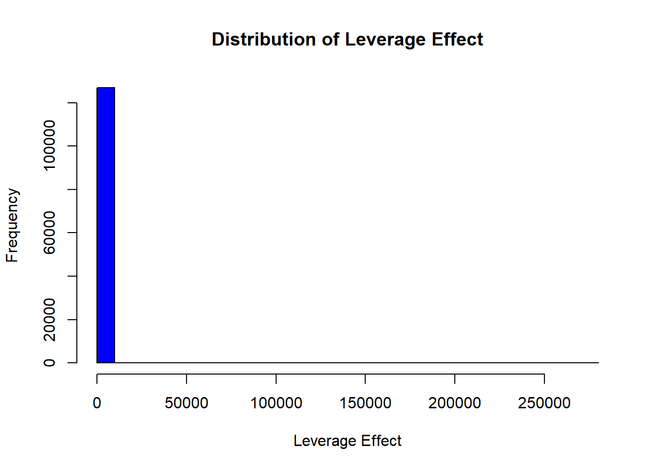
# Plot histogram of leverage effect
hist(
df_leverage_effect$leverage_effect,
main = "Distribution of Leverage Effect",
xlab = "Leverage Effect",
col = "blue",
breaks = 30
)
# Compute coefficient of variation (CV)
cv_le <-
sd(df_leverage_effect$leverage_effect, na.rm = TRUE) / mean_le * 100
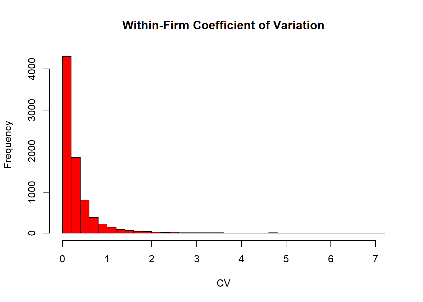
# Plot within-firm coefficient of variation histogram
df_leverage_effect %>%
group_by(gvkey) %>%
slice(1) %>%
ungroup() %>%
mutate(cv = within_sd_le / within_mean_le) %>%
pull(cv) %>%
hist(
main = "Within-Firm Coefficient of Variation",
xlab = "CV",
col = "red",
breaks = 30
)