7.3 Binomial Regression
In previous sections, we introduced binomial regression models, including both Logistic Regression and probit regression, and discussed their theoretical foundations. Now, we apply these methods to real-world data using the esoph dataset, which examines the relationship between esophageal cancer and potential risk factors such as alcohol consumption and age group.
7.3.1 Dataset Overview
The esoph dataset consists of:
Successes (
ncases): The number of individuals diagnosed with esophageal cancer.Failures (
ncontrols): The number of individuals in the control group (without cancer).Predictors:
agegp: Age group of individuals.alcgp: Alcohol consumption category.tobgp: Tobacco consumption category.
Before fitting our models, let’s inspect the dataset and visualize some key relationships.
# Load and inspect the dataset
data("esoph")
head(esoph, n = 3)
#>   agegp     alcgp    tobgp ncases ncontrols
#> 1 25-34 0-39g/day 0-9g/day      0        40
#> 2 25-34 0-39g/day    10-19      0        10
#> 3 25-34 0-39g/day    20-29      0         6
# Visualizing the proportion of cancer cases by alcohol consumption
plot(
esoph$ncases / (esoph$ncases + esoph$ncontrols) ~ esoph$alcgp,
ylab = "Proportion of Cancer Cases",
xlab = "Alcohol Consumption Group",
main = "Esophageal Cancer Data"
)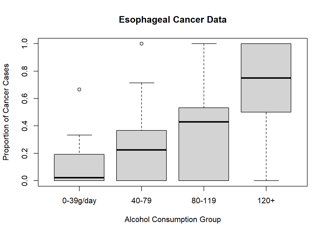
Figure 7.6: Esophageal Cancer Data
7.3.2 Apply Logistic Model
We first fit a logistic regression model, where the response variable is the proportion of cancer cases (ncases) relative to total observations (ncases + ncontrols).
# Logistic regression using alcohol consumption as a predictor
model <-
    glm(cbind(ncases, ncontrols) ~ alcgp,
        data = esoph,
        family = binomial)

# Summary of the model
summary(model)
#>
#> Call:
#> glm(formula = cbind(ncases, ncontrols) ~ alcgp, family = binomial,
#>     data = esoph)
#>
#> Coefficients:
#>             Estimate Std. Error z value Pr(>|z|)
#> (Intercept)  -2.5885     0.1925 -13.444  < 2e-16 ***
#> alcgp40-79    1.2712     0.2323   5.472 4.46e-08 ***
#> alcgp80-119   2.0545     0.2611   7.868 3.59e-15 ***
#> alcgp120+     3.3042     0.3237  10.209  < 2e-16 ***
#> ---
#> Signif. codes:  0 '***' 0.001 '**' 0.01 '*' 0.05 '.' 0.1 ' ' 1
#>
#> (Dispersion parameter for binomial family taken to be 1)
#>
#>     Null deviance: 367.95  on 87  degrees of freedom
#> Residual deviance: 221.46  on 84  degrees of freedom
#> AIC: 344.51
#>
#> Number of Fisher Scoring iterations: 5
Interpretation
The coefficients represent the log-odds of having esophageal cancer relative to the baseline alcohol consumption group.
P-values indicate whether alcohol consumption levels significantly influence cancer risk.
Model Diagnostics
# Convert coefficients to odds ratios
exp(coefficients(model))
#> (Intercept)  alcgp40-79 alcgp80-119   alcgp120+
#>  0.07512953  3.56527094  7.80261593 27.22570533

# Model goodness-of-fit measures
deviance(model) / df.residual(model)  # Closer to 1 suggests a better fit
#> [1] 2.63638
model$aic  # Lower AIC is preferable for model comparison
#> [1] 344.5109
To improve our model, we include age group (agegp) as an additional predictor.
# Logistic regression with alcohol consumption and age
better_model <- glm(
    cbind(ncases, ncontrols) ~ agegp + alcgp,
    data = esoph,
    family = binomial
)

# Summary of the improved model
summary(better_model)
#>
#> Call:
#> glm(formula = cbind(ncases, ncontrols) ~ agegp + alcgp, family = binomial,
#>     data = esoph)
#>
#> Coefficients:
#>             Estimate Std. Error z value Pr(>|z|)
#> (Intercept)  -6.1472     1.0419  -5.900 3.63e-09 ***
#> agegp35-44    1.6311     1.0800   1.510 0.130973
#> agegp45-54    3.4258     1.0389   3.297 0.000976 ***
#> agegp55-64    3.9435     1.0346   3.811 0.000138 ***
#> agegp65-74    4.3568     1.0413   4.184 2.87e-05 ***
#> agegp75+      4.4242     1.0914   4.054 5.04e-05 ***
#> alcgp40-79    1.4343     0.2448   5.859 4.64e-09 ***
#> alcgp80-119   2.0071     0.2776   7.230 4.84e-13 ***
#> alcgp120+     3.6800     0.3763   9.778  < 2e-16 ***
#> ---
#> Signif. codes:  0 '***' 0.001 '**' 0.01 '*' 0.05 '.' 0.1 ' ' 1
#>
#> (Dispersion parameter for binomial family taken to be 1)
#>
#>     Null deviance: 367.95  on 87  degrees of freedom
#> Residual deviance: 105.88  on 79  degrees of freedom
#> AIC: 238.94
#>
#> Number of Fisher Scoring iterations: 6

# Model evaluation
better_model$aic # Lower AIC is better
#> [1] 238.9361

# Convert coefficients to odds ratios
# exp(coefficients(better_model))
data.frame(`Odds Ratios` = exp(coefficients(better_model)))
#>              Odds.Ratios
#> (Intercept)  0.002139482
#> agegp35-44   5.109601844
#> agegp45-54  30.748594216
#> agegp55-64  51.596634690
#> agegp65-74  78.005283850
#> agegp75+    83.448437749
#> alcgp40-79   4.196747169
#> alcgp80-119  7.441782227
#> alcgp120+   39.646885126

# Compare models using likelihood ratio test (Chi-square test)
pchisq(
    q = model$deviance - better_model$deviance,
    df = model$df.residual - better_model$df.residual,
    lower.tail = FALSE
)
#> [1] 2.713923e-23
Key Takeaways
AIC Reduction: A lower AIC suggests that adding age as a predictor improves the model.
Likelihood Ratio Test: This test compares the two models and determines whether the improvement is statistically significant.
7.3.3 Apply Probit Model
As discussed earlier, the probit model is an alternative to logistic regression, using a cumulative normal distribution instead of the logistic function.
# Probit regression model
Prob_better_model <- glm(
    cbind(ncases, ncontrols) ~ agegp + alcgp,
    data = esoph,
    family = binomial(link = probit)
)

# Summary of the probit model
summary(Prob_better_model)
#>
#> Call:
#> glm(formula = cbind(ncases, ncontrols) ~ agegp + alcgp, family = binomial(link = probit),
#>     data = esoph)
#>
#> Coefficients:
#>             Estimate Std. Error z value Pr(>|z|)
#> (Intercept)  -3.3741     0.4922  -6.855 7.13e-12 ***
#> agegp35-44    0.8562     0.5081   1.685 0.092003 .
#> agegp45-54    1.7829     0.4904   3.636 0.000277 ***
#> agegp55-64    2.1034     0.4876   4.314 1.61e-05 ***
#> agegp65-74    2.3374     0.4930   4.741 2.13e-06 ***
#> agegp75+      2.3694     0.5275   4.491 7.08e-06 ***
#> alcgp40-79    0.8080     0.1330   6.076 1.23e-09 ***
#> alcgp80-119   1.1399     0.1558   7.318 2.52e-13 ***
#> alcgp120+     2.1204     0.2060  10.295  < 2e-16 ***
#> ---
#> Signif. codes:  0 '***' 0.001 '**' 0.01 '*' 0.05 '.' 0.1 ' ' 1
#>
#> (Dispersion parameter for binomial family taken to be 1)
#>
#>     Null deviance: 367.95  on 87  degrees of freedom
#> Residual deviance: 104.48  on 79  degrees of freedom
#> AIC: 237.53
#>
#> Number of Fisher Scoring iterations: 6
Why Consider a Probit Model?
Like logistic regression, probit regression estimates probabilities, but it assumes a normal distribution of the latent variable.
While the interpretation of coefficients differs, model comparisons can still be made using AIC.