9.6 Application: Nonlinear and Generalized Linear Mixed Models
9.6.1 Binomial Data: CBPP Dataset
We will use the CBPP dataset from the lme4 package to demonstrate different estimation approaches for binomial mixed models.
library(lme4)
data(cbpp, package = "lme4")
head(cbpp)
#>   herd incidence size period
#> 1    1         2   14      1
#> 2    1         3   12      2
#> 3    1         4    9      3
#> 4    1         0    5      4
#> 5    2         3   22      1
#> 6    2         1   18      2
The data contain information about contagious bovine pleuropneumonia (CBPP) cases across different herds and periods.
- Penalized Quasi-Likelihood
Pros:
Linearizes the response to create a pseudo-response, similar to linear mixed models.
Computationally efficient.
Cons:
Biased for binary or Poisson data with small counts.
Random effects must be interpreted on the link scale.
AIC/BIC values are not interpretable since PQL does not rely on full likelihood.
library(MASS)
pql_cbpp <- glmmPQL(
    cbind(incidence, size - incidence) ~ period,
    random  = ~ 1 | herd,
    data    = cbpp,
    family  = binomial(link = "logit"),
    verbose = FALSE
)
summary(pql_cbpp)
#> Linear mixed-effects model fit by maximum likelihood
#>   Data: cbpp
#>   AIC BIC logLik
#>    NA  NA     NA
#>
#> Random effects:
#>  Formula: ~1 | herd
#>         (Intercept) Residual
#> StdDev:   0.5563535 1.184527
#>
#> Variance function:
#>  Structure: fixed weights
#>  Formula: ~invwt
#> Fixed effects:  cbind(incidence, size - incidence) ~ period
#>                 Value Std.Error DF   t-value p-value
#> (Intercept) -1.327364 0.2390194 38 -5.553372  0.0000
#> period2     -1.016126 0.3684079 38 -2.758156  0.0089
#> period3     -1.149984 0.3937029 38 -2.920944  0.0058
#> period4     -1.605217 0.5178388 38 -3.099839  0.0036
#>  Correlation:
#>         (Intr) perid2 perid3
#> period2 -0.399
#> period3 -0.373  0.260
#> period4 -0.282  0.196  0.182
#>
#> Standardized Within-Group Residuals:
#>        Min         Q1        Med         Q3        Max
#> -2.0591168 -0.6493095 -0.2747620  0.5170492  2.6187632
#>
#> Number of Observations: 56
#> Number of Groups: 15
Interpretation
The above result shows how herd-specific odds vary, accounting for random effects.
The fixed effects are interpreted similarly to logistic regression. For example, with the logit link:
- The log odds of having a case in period 2 are -1.016 less than in period 1 (baseline).
summary(pql_cbpp)$tTable
#>                 Value Std.Error DF   t-value      p-value
#> (Intercept) -1.327364 0.2390194 38 -5.553372 2.333216e-06
#> period2     -1.016126 0.3684079 38 -2.758156 8.888179e-03
#> period3     -1.149984 0.3937029 38 -2.920944 5.843007e-03
#> period4 -1.605217 0.5178388 38 -3.099839 3.637000e-03- Numerical Integration with
glmer
Pros:
- More accurate estimation since the method directly integrates over random effects.
Cons:
Computationally more expensive, especially with high-dimensional random effects.
May struggle with convergence for complex models.
numint_cbpp <- glmer(
    cbind(incidence, size - incidence) ~ period + (1 | herd),
    data = cbpp,
    family = binomial(link = "logit")
)
summary(numint_cbpp)
#> Generalized linear mixed model fit by maximum likelihood (Laplace
#>   Approximation) [glmerMod]
#>  Family: binomial  ( logit )
#> Formula: cbind(incidence, size - incidence) ~ period + (1 | herd)
#>    Data: cbpp
#>
#>       AIC       BIC    logLik -2*log(L)  df.resid
#>     194.1     204.2     -92.0     184.1        51
#>
#> Scaled residuals:
#>     Min      1Q  Median      3Q     Max
#> -2.3816 -0.7889 -0.2026  0.5142  2.8791
#>
#> Random effects:
#>  Groups Name        Variance Std.Dev.
#>  herd   (Intercept) 0.4123   0.6421
#> Number of obs: 56, groups:  herd, 15
#>
#> Fixed effects:
#>             Estimate Std. Error z value Pr(>|z|)
#> (Intercept)  -1.3983     0.2312  -6.048 1.47e-09 ***
#> period2      -0.9919     0.3032  -3.272 0.001068 **
#> period3      -1.1282     0.3228  -3.495 0.000474 ***
#> period4      -1.5797     0.4220  -3.743 0.000182 ***
#> ---
#> Signif. codes:  0 '***' 0.001 '**' 0.01 '*' 0.05 '.' 0.1 ' ' 1
#>
#> Correlation of Fixed Effects:
#>         (Intr) perid2 perid3
#> period2 -0.363
#> period3 -0.340  0.280
#> period4 -0.260  0.213  0.198
Comparing PQL and Numerical Integration
For small datasets, the difference between PQL and numerical integration may be minimal.
library(rbenchmark)
benchmark(
    "PQL (MASS)" = {
        glmmPQL(
            cbind(incidence, size - incidence) ~ period,
            random = ~ 1 | herd,
            data = cbpp,
            family = binomial(link = "logit"),
            verbose = FALSE
        )
    },
    "Numerical Integration (lme4)" = {
        glmer(
            cbind(incidence, size - incidence) ~ period + (1 | herd),
            data = cbpp,
            family = binomial(link = "logit")
        )
    },
    replications = 50,
    columns = c("test", "replications", "elapsed", "relative"),
    order = "relative"
)
#>                           test replications elapsed relative
#> 1                   PQL (MASS)           50    4.36     1.00
#> 2 Numerical Integration (lme4)           50    8.98     2.06
Improving Accuracy with Gauss-Hermite Quadrature
Setting nAGQ > 1 increases the accuracy of the likelihood approximation:
numint_cbpp_GH <- glmer(
    cbind(incidence, size - incidence) ~ period + (1 | herd),
    data = cbpp,
    family = binomial(link = "logit"),
    nAGQ = 20
)
summary(numint_cbpp_GH)$coefficients[, 1] -
    summary(numint_cbpp)$coefficients[, 1]
#>   (Intercept)       period2       period3       period4
#> -0.0008808634 0.0005160912 0.0004066218 0.0002644629- Bayesian Approach with
MCMCglmm
Pros:
Incorporates prior information and handles complex models with intractable likelihoods.
Provides full posterior distributions for parameters.
Cons:
- Computationally intensive, especially with large datasets or complex hierarchical structures.
library(MCMCglmm)
Bayes_cbpp <- MCMCglmm(
    cbind(incidence, size - incidence) ~ period,
    random = ~ herd,
    data = cbpp,
    family = "multinomial2",
    verbose = FALSE
)
summary(Bayes_cbpp)
#>
#>  Iterations = 3001:12991
#>  Thinning interval  = 10
#>  Sample size  = 1000
#>
#>  DIC: 540.0825
#>
#>  G-structure:  ~herd
#>
#>      post.mean  l-95% CI u-95% CI eff.samp
#> herd   0.07063 9.692e-17   0.5178    24.21
#>
#>  R-structure:  ~units
#>
#>       post.mean l-95% CI u-95% CI eff.samp
#> units     1.019 0.001394    1.994    41.46
#>
#>  Location effects: cbind(incidence, size - incidence) ~ period
#>
#>             post.mean l-95% CI u-95% CI eff.samp  pMCMC
#> (Intercept)   -1.5184  -2.1070  -0.8563    866.8 <0.001 ***
#> period2       -1.2384  -2.1924  -0.2763    814.4  0.022 *
#> period3       -1.3623  -2.4241  -0.3404    423.5  0.012 *
#> period4       -2.0180  -3.3176  -0.9533    376.5 <0.001 ***
#> ---
#> Signif. codes: 0 '***' 0.001 '**' 0.01 '*' 0.05 '.' 0.1 ' ' 1MCMCglmmfits a residual variance component (useful with dispersion issues).
Variance Component Analysis
Posterior Summaries
summary(Bayes_cbpp)$solutions
#>             post.mean  l-95% CI   u-95% CI eff.samp pMCMC
#> (Intercept) -1.518387 -2.107027 -0.8563162 866.8111 0.001
#> period2     -1.238402 -2.192393 -0.2762579 814.3531 0.022
#> period3     -1.362322 -2.424085 -0.3403704 423.4672 0.012
#> period4     -2.018006 -3.317563 -0.9533247 376.4856 0.001
MCMC Diagnostics
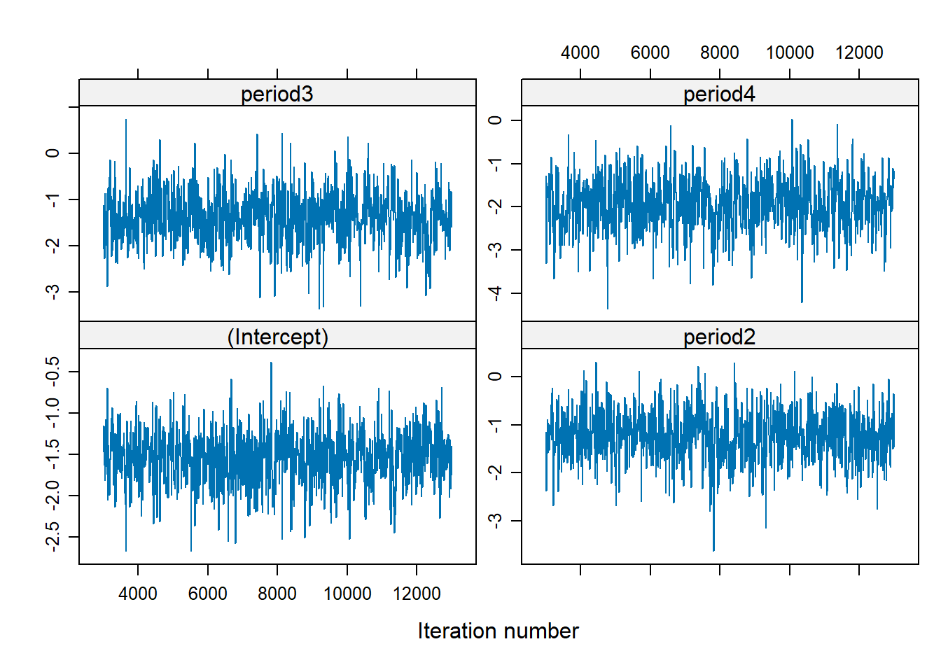
Figure 9.1: MCMC Diagnostic
There is no trend (i.e., well-mixed).
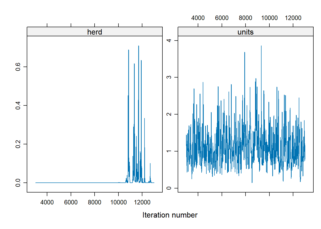
Figure 9.2: Variable MCMC Diagnostic
For the herd variable, many of the values are 0, which suggests a problem. To address the instability in the herd effect sampling, we can either:
Modify prior distributions,
Increase the number of iterations
Bayes_cbpp2 <- MCMCglmm(
    cbind(incidence, size - incidence) ~ period,
    random = ~ herd,
    data = cbpp,
    family = "multinomial2",
    nitt = 20000,
    burnin = 10000,
    prior = list(G = list(list(V = 1, nu = 0.1))),
    verbose = FALSE
)
xyplot(as.mcmc(Bayes_cbpp2$VCV), layout = c(2, 1))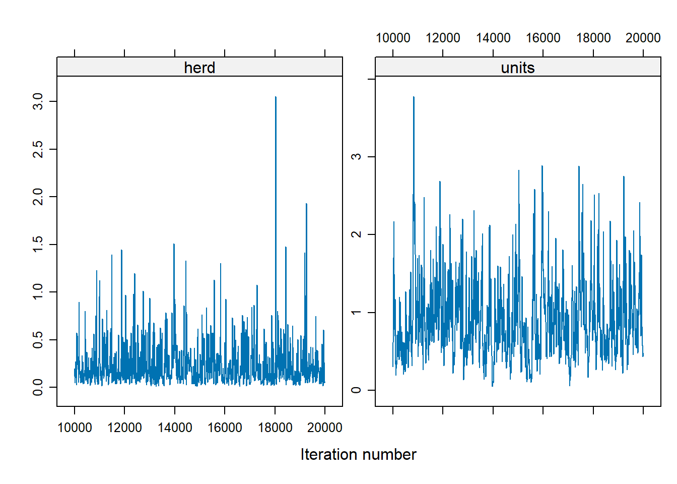
Figure 9.3: Variable MCMC Diagnostic (Alternative)
To change the shape of priors, in MCMCglmm use:
Vcontrols for the location of the distribution (default = 1)nucontrols for the concentration around V (default = 0)
9.6.2 Count Data: Owl Dataset
We’ll now model count data using the Owl dataset
library(glmmTMB)
library(dplyr)
data(Owls, package = "glmmTMB")
Owls <- Owls %>% rename(Ncalls = SiblingNegotiation)- Poisson GLMM
Modeling call counts with a Poisson distribution:
In a typical Poisson model, the Poisson mean \(\lambda\) is modeled as: \[ \log(\lambda) = x' \beta \] However, if the response variable represents a rate (e.g., counts per BroodSize), we can model it as: \[ \log\left(\frac{\lambda}{b}\right) = x' \beta \] This is equivalent to: \[ \log(\lambda) = \log(b) + x' \beta \] where \(b\) represents BroodSize. In this formulation, we “offset” the mean by including the logarithm of \(b\) as an offset term in the model. This adjustment accounts for the varying exposure or denominator in rate-based responses.
owls_glmer <- glmer(
    Ncalls ~ offset(log(BroodSize)) + FoodTreatment * SexParent + (1 | Nest),
    family = poisson,
    data = Owls
)
summary(owls_glmer)
#> Generalized linear mixed model fit by maximum likelihood (Laplace
#>   Approximation) [glmerMod]
#>  Family: poisson  ( log )
#> Formula: Ncalls ~ offset(log(BroodSize)) + FoodTreatment * SexParent +
#>     (1 | Nest)
#>    Data: Owls
#>
#>       AIC       BIC    logLik -2*log(L)  df.resid
#>    5212.8    5234.8   -2601.4    5202.8       594
#>
#> Scaled residuals:
#>     Min      1Q  Median      3Q     Max
#> -3.5529 -1.7971 -0.6842  1.2689 11.4312
#>
#> Random effects:
#>  Groups Name        Variance Std.Dev.
#>  Nest   (Intercept) 0.2063   0.4542
#> Number of obs: 599, groups:  Nest, 27
#>
#> Fixed effects:
#>                                     Estimate Std. Error z value Pr(>|z|)
#> (Intercept)                          0.65585    0.09567   6.855 7.12e-12 ***
#> FoodTreatmentSatiated               -0.65612    0.05606 -11.705  < 2e-16 ***
#> SexParentMale                       -0.03705    0.04501  -0.823   0.4104
#> FoodTreatmentSatiated:SexParentMale  0.13135    0.07036   1.867   0.0619 .
#> ---
#> Signif. codes:  0 '***' 0.001 '**' 0.01 '*' 0.05 '.' 0.1 ' ' 1
#>
#> Correlation of Fixed Effects:
#>             (Intr) FdTrtS SxPrnM
#> FdTrtmntStt -0.225
#> SexParentMl -0.292  0.491
#> FdTrtmS:SPM 0.170 -0.768 -0.605- Nest explains a relatively large proportion of the variability (its standard deviation is larger than some coefficients).
- The model fit isn’t great (deviance of 5202 on 594 df).
- Negative Binomial Model
Addressing overdispersion using the negative binomial distribution:
owls_glmerNB <- glmer.nb(
    Ncalls ~ offset(log(BroodSize)) + FoodTreatment * SexParent + (1 | Nest),
    data = Owls
)
summary(owls_glmerNB)
#> Generalized linear mixed model fit by maximum likelihood (Laplace
#>   Approximation) [glmerMod]
#>  Family: Negative Binomial(0.8423)  ( log )
#> Formula: Ncalls ~ offset(log(BroodSize)) + FoodTreatment * SexParent +
#>     (1 | Nest)
#>    Data: Owls
#>
#>       AIC       BIC    logLik -2*log(L)  df.resid
#>    3495.6    3522.0   -1741.8    3483.6       593
#>
#> Scaled residuals:
#>     Min      1Q  Median      3Q     Max
#> -0.8859 -0.7737 -0.2701  0.4443  6.1432
#>
#> Random effects:
#>  Groups Name        Variance Std.Dev.
#>  Nest   (Intercept) 0.1245   0.3529
#> Number of obs: 599, groups:  Nest, 27
#>
#> Fixed effects:
#>                                     Estimate Std. Error z value Pr(>|z|)
#> (Intercept)                          0.69005    0.13400   5.150 2.61e-07 ***
#> FoodTreatmentSatiated               -0.76657    0.16509  -4.643 3.43e-06 ***
#> SexParentMale                       -0.02605    0.14575  -0.179    0.858
#> FoodTreatmentSatiated:SexParentMale  0.15680    0.20512   0.764    0.445
#> ---
#> Signif. codes:  0 '***' 0.001 '**' 0.01 '*' 0.05 '.' 0.1 ' ' 1
#>
#> Correlation of Fixed Effects:
#>             (Intr) FdTrtS SxPrnM
#> FdTrtmntStt -0.602
#> SexParentMl -0.683  0.553
#> FdTrtmS:SPM  0.450 -0.744 -0.671
There is an improvement using negative binomial considering over-dispersion
library(ggplot2)
ggplot(Owls, aes(x = Ncalls)) +
  geom_histogram(
    bins = 30,
    fill = "steelblue",
    color = "white",
    alpha = 0.8
  ) +
  labs(title = "Distribution of Owl Call Counts",
       x = "Number of Calls",
       y = "Frequency") +
  theme_minimal(base_size = 14)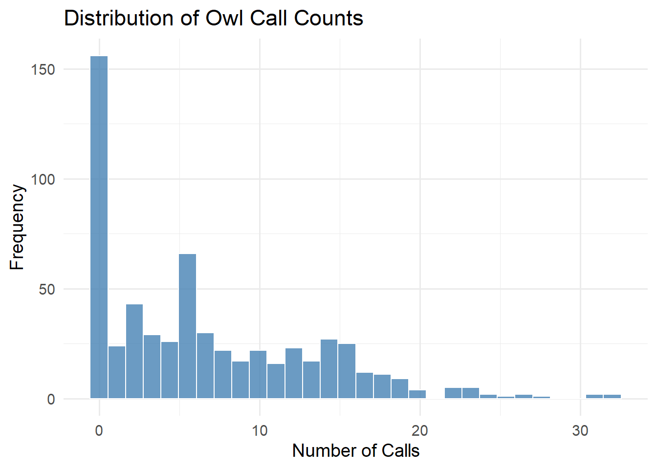
Figure 9.4: Distribution of Owl Call Counts
- Zero-Inflated Model
Handling excess zeros with a zero-inflated Poisson model:
library(glmmTMB)
owls_glmm <-
    glmmTMB(
        Ncalls ~ FoodTreatment * SexParent + offset(log(BroodSize)) +
            (1 | Nest),
        ziformula =  ~ 0,
        family = nbinom2(link = "log"),
        data = Owls
    )
owls_glmm_zi <-
    glmmTMB(
        Ncalls ~ FoodTreatment * SexParent + offset(log(BroodSize)) +
            (1 | Nest),
        ziformula =  ~ 1,
        family = nbinom2(link = "log"),
        data = Owls
    )

# Scale Arrival time to use as a covariate for zero-inflation parameter
Owls$ArrivalTime <- scale(Owls$ArrivalTime)
owls_glmm_zi_cov <- glmmTMB(
    Ncalls ~ FoodTreatment * SexParent +
        offset(log(BroodSize)) +
        (1 | Nest),
    ziformula =  ~ ArrivalTime,
    family = nbinom2(link = "log"),
    data = Owls
)

as.matrix(anova(owls_glmm, owls_glmm_zi))
#>              Df      AIC      BIC    logLik deviance    Chisq Chi Df
#> owls_glmm     6 3495.610 3521.981 -1741.805 3483.610       NA     NA
#> owls_glmm_zi  7 3431.646 3462.413 -1708.823 3417.646 65.96373      1
#>                Pr(>Chisq)
#> owls_glmm              NA
#> owls_glmm_zi 4.592983e-16


as.matrix(anova(owls_glmm_zi, owls_glmm_zi_cov))
#>                  Df      AIC      BIC    logLik deviance    Chisq Chi Df
#> owls_glmm_zi      7 3431.646 3462.413 -1708.823 3417.646       NA     NA
#> owls_glmm_zi_cov  8 3422.532 3457.694 -1703.266 3406.532 11.11411      1
#>                    Pr(>Chisq)
#> owls_glmm_zi               NA
#> owls_glmm_zi_cov 0.0008567362


summary(owls_glmm_zi_cov)
#>  Family: nbinom2  ( log )
#> Formula:
#> Ncalls ~ FoodTreatment * SexParent + offset(log(BroodSize)) +      (1 | Nest)
#> Zero inflation:          ~ArrivalTime
#> Data: Owls
#>
#>       AIC       BIC    logLik -2*log(L)  df.resid
#>    3422.5    3457.7   -1703.3    3406.5       591
#>
#> Random effects:
#>
#> Conditional model:
#>  Groups Name        Variance Std.Dev.
#>  Nest   (Intercept) 0.07487  0.2736
#> Number of obs: 599, groups:  Nest, 27
#>
#> Dispersion parameter for nbinom2 family (): 2.22
#>
#> Conditional model:
#>                                     Estimate Std. Error z value Pr(>|z|)
#> (Intercept)                          0.84778    0.09961   8.511  < 2e-16 ***
#> FoodTreatmentSatiated               -0.39529    0.13742  -2.877  0.00402 **
#> SexParentMale                       -0.07025    0.10435  -0.673  0.50079
#> FoodTreatmentSatiated:SexParentMale  0.12388    0.16449   0.753  0.45138
#> ---
#> Signif. codes:  0 '***' 0.001 '**' 0.01 '*' 0.05 '.' 0.1 ' ' 1
#>
#> Zero-inflation model:
#>             Estimate Std. Error z value Pr(>|z|)
#> (Intercept)  -1.3018     0.1261  -10.32  < 2e-16 ***
#> ArrivalTime   0.3545     0.1074    3.30 0.000966 ***
#> ---
#> Signif. codes:  0 '***' 0.001 '**' 0.01 '*' 0.05 '.' 0.1 ' ' 1
glmmTMB can handle ZIP GLMMs since it adds automatic differentiation to existing estimation strategies.
We can see ZIP GLMM with an arrival time covariate on the zero is best.
Arrival time has a positive effect on observing a nonzero number of calls
Interactions are non significant, the food treatment is significant (fewer calls after eating)
Nest variability is large in magnitude (without this, the parameter estimates change)
9.6.3 Binomial Example: Gotway Hessian Fly Data
We will analyze the Gotway Hessian Fly dataset from the agridat package to model binomial outcomes using both frequentist and Bayesian approaches.
9.6.3.1 Data Visualization
library(agridat)
library(ggplot2)
library(lme4)
library(spaMM)

data(gotway.hessianfly)
dat <- gotway.hessianfly
dat$prop <- dat$y / dat$n # Proportion of successesggplot(dat, aes(x = lat, y = long, fill = prop)) +
geom_tile() +
scale_fill_gradient(low = 'white', high = 'black') +
geom_text(aes(label = gen, color = block)) +
ggtitle('Gotway Hessian Fly: Proportion of Infestation')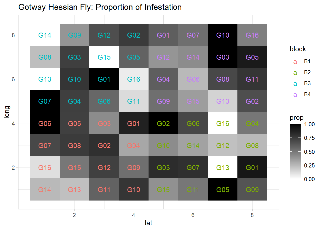
Figure 9.5: Gotway Hessian Fly: Proportion of Infestation
9.6.3.2 Model Specification
Fixed Effects (\(\boldsymbol{\beta}\)): Genotype (
gen)Random Effects (\(\boldsymbol{\alpha}\)): Block (
block), accounting for spatial or experimental design variability
- Frequentist Approach with
glmer
flymodel <- glmer(
    cbind(y, n - y) ~ gen + (1 | block),
    data   = dat,
    family = binomial,
    nAGQ   = 5  # Using adaptive Gauss-Hermite quadrature for accuracy
)
summary(flymodel)
#> Generalized linear mixed model fit by maximum likelihood (Adaptive
#>   Gauss-Hermite Quadrature, nAGQ = 5) [glmerMod]
#>  Family: binomial  ( logit )
#> Formula: cbind(y, n - y) ~ gen + (1 | block)
#>    Data: dat
#>
#>       AIC       BIC    logLik -2*log(L)  df.resid
#>     162.2     198.9     -64.1     128.2        47
#>
#> Scaled residuals:
#>      Min       1Q   Median       3Q      Max
#> -2.38644 -1.01188  0.09631  1.03468  2.75479
#>
#> Random effects:
#>  Groups Name        Variance Std.Dev.
#>  block  (Intercept) 0.001022 0.03196
#> Number of obs: 64, groups:  block, 4
#>
#> Fixed effects:
#>             Estimate Std. Error z value Pr(>|z|)
#> (Intercept)   1.5035     0.3914   3.841 0.000122 ***
#> genG02       -0.1939     0.5302  -0.366 0.714645
#> genG03       -0.5408     0.5103  -1.060 0.289263
#> genG04       -1.4342     0.4714  -3.043 0.002346 **
#> genG05       -0.2037     0.5429  -0.375 0.707487
#> genG06       -0.9783     0.5046  -1.939 0.052534 .
#> genG07       -0.6041     0.5111  -1.182 0.237237
#> genG08       -1.6774     0.4907  -3.418 0.000630 ***
#> genG09       -1.3984     0.4725  -2.960 0.003079 **
#> genG10       -0.6817     0.5333  -1.278 0.201183
#> genG11       -1.4630     0.4843  -3.021 0.002522 **
#> genG12       -1.4591     0.4918  -2.967 0.003010 **
#> genG13       -3.5528     0.6600  -5.383 7.31e-08 ***
#> genG14       -2.5073     0.5264  -4.763 1.90e-06 ***
#> genG15       -2.0872     0.4851  -4.302 1.69e-05 ***
#> genG16       -2.9697     0.5383  -5.517 3.46e-08 ***
#> ---
#> Signif. codes: 0 '***' 0.001 '**' 0.01 '*' 0.05 '.' 0.1 ' ' 1Interpretation:
The fixed effects (
gen) indicate how different genotypes influence the infestation probability.The random effect for
blockcaptures variability due to experimental blocks, improving model robustness.Odds Ratios: Exponentiating coefficients helps interpret the impact on infestation odds.
- Bayesian Approach with
MCMCglmm
library(MCMCglmm)
library(coda)

Bayes_flymodel <- MCMCglmm(
    cbind(y, n - y) ~ gen,
    random  = ~ block,
    data    = dat,
    family  = "multinomial2",
    verbose = FALSE
)
summary(Bayes_flymodel)
#>
#>  Iterations = 3001:12991
#>  Thinning interval  = 10
#>  Sample size  = 1000
#>
#>  DIC: 877.1775
#>
#>  G-structure:  ~block
#>
#>       post.mean  l-95% CI u-95% CI eff.samp
#> block   0.01214 5.472e-17  0.01668    791.1
#>
#>  R-structure:  ~units
#>
#>       post.mean l-95% CI u-95% CI eff.samp
#> units     1.067   0.3361    1.941    485.2
#>
#>  Location effects: cbind(y, n - y) ~ gen
#>
#>             post.mean l-95% CI u-95% CI eff.samp  pMCMC
#> (Intercept)   1.99591  0.65346  3.41779    826.3  0.010 *
#> genG02       -0.41965 -2.28157  1.41017    908.7  0.666
#> genG03       -0.76976 -2.86277  1.06801   1000.0  0.434
#> genG04       -1.85788 -3.86373 -0.04027    848.0  0.060 .
#> genG05       -0.39076 -2.40421  1.44283   1000.0  0.716
#> genG06       -1.31857 -3.24040  0.48095    818.5  0.162
#> genG07       -0.79303 -2.66806  1.10452   1000.0  0.388
#> genG08       -2.12004 -3.93637 -0.31697    729.3  0.022 *
#> genG09       -1.89865 -3.65747 -0.18248   1000.0  0.032 *
#> genG10       -0.83074 -2.57605  1.23376    839.1  0.402
#> genG11       -2.01243 -4.07204 -0.28634    586.4  0.034 *
#> genG12       -1.96678 -3.77565 -0.14728   1000.0  0.040 *
#> genG13       -4.48060 -6.64994 -2.26667    693.0 <0.001 ***
#> genG14       -3.26123 -5.25412 -1.47261    633.8 <0.001 ***
#> genG15       -2.83491 -4.85355 -0.95720    774.5  0.006 **
#> genG16       -3.93455 -6.07112 -1.94770    657.9 <0.001 ***
#> ---
#> Signif. codes:  0 '***' 0.001 '**' 0.01 '*' 0.05 '.' 0.1 ' ' 1
MCMC Diagnostics
Trace Plot: Checks for chain mixing and convergence.
Autocorrelation Plot: Evaluates dependency between MCMC samples.
# Trace plot for the first fixed effect
plot(Bayes_flymodel$Sol[, 1],
     main = colnames(Bayes_flymodel$Sol)[1])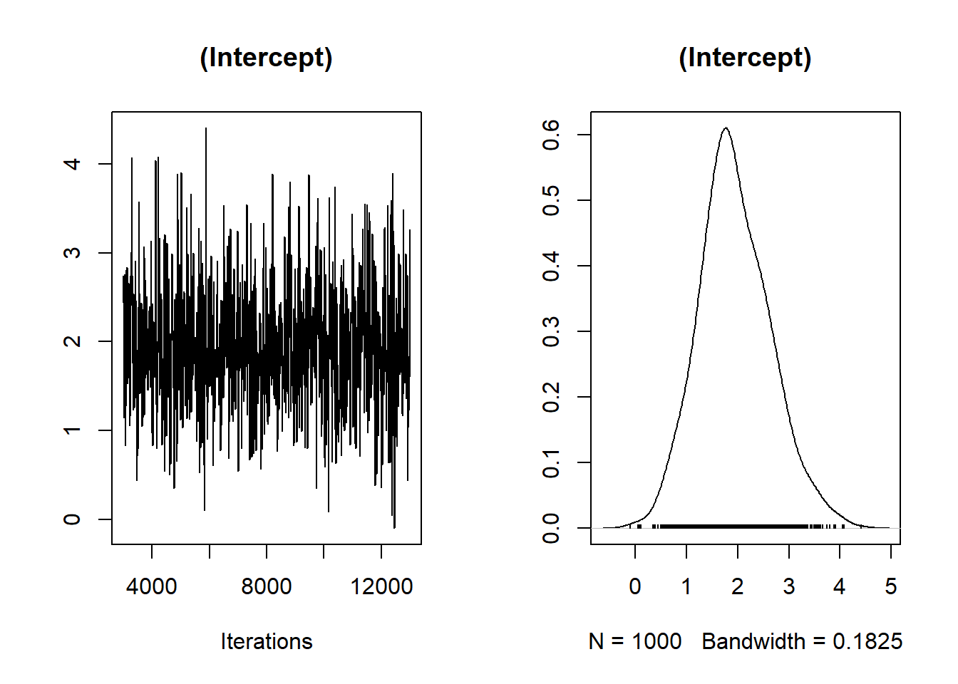
Figure 9.6: Trace Plot
# Autocorrelation plot
autocorr.plot(Bayes_flymodel$Sol[, 1],
              main = colnames(Bayes_flymodel$Sol)[1])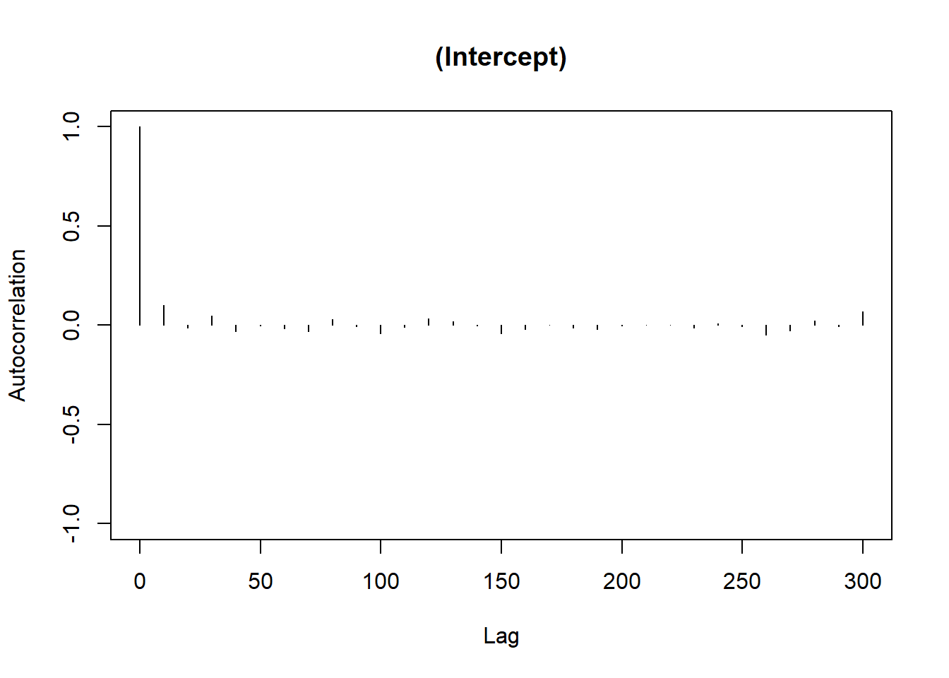
Figure 9.7: Autocorrelation Plot
Bayesian Interpretation:
Posterior Means: Represent the central tendency of the parameter estimates.
Credible Intervals: Unlike frequentist confidence intervals, they can be interpreted directly as the probability that the parameter lies within the interval.
9.6.4 Nonlinear Mixed Model: Yellow Poplar Data
This dataset comes from Schabenberger and Pierce (2001)
9.6.4.2 Data Visualization
library(dplyr)

dat2 <- dat2 %>% group_by(tn) %>% mutate(
    z = case_when(
        totht < 74 ~ 'a: 0-74ft',
        totht < 88 ~ 'b: 74-88',
        totht < 95 ~ 'c: 88-95',
        totht < 99 ~ 'd: 95-99',
        totht < 104 ~ 'e: 99-104',
        totht < 109 ~ 'f: 104-109',
        totht < 115 ~ 'g: 109-115',
        totht < 120 ~ 'h: 115-120',
        totht < 140 ~ 'i: 120-150',
        TRUE ~ 'j: 150+'
    )
)ggplot(dat2, aes(x = r, y = cumv)) +
geom_point(size = 0.5) +
facet_wrap(vars(z)) +
labs(title = "Cumulative Volume vs. Relative Height by Tree Height Group")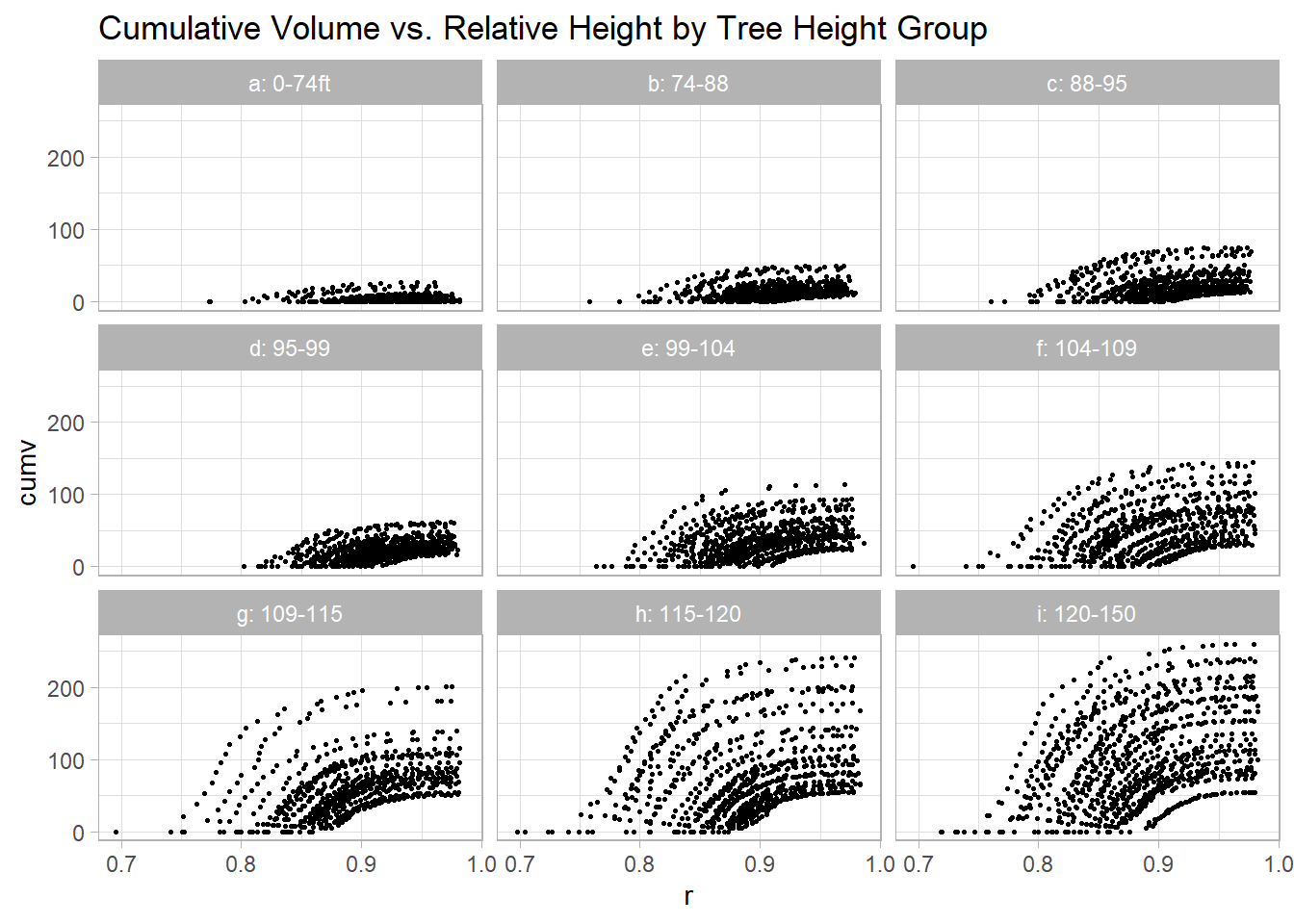
Figure 9.8: Cumulative Volume vs. Relative Height by Tree Height Group
9.6.4.3 Model Specification
The proposed Nonlinear Mixed Model is: \[ V_{ij} = \left(\beta_0 + (\beta_1 + b_{1i})\frac{D_i^2 H_i}{1000}\right) \exp\left[-(\beta_2 + b_{2i}) t_{ij} \exp(\beta_3 t_{ij})\right] + e_{ij} \] Where:
\(b_{1i}, b_{2i}\) are random effects for tree \(i\).
\(e_{ij}\) are residual errors.
9.6.4.4 Fitting the Nonlinear Mixed Model
library(nlme)

tmp <- nlme(
    cumv ~ (b0 + (b1 + u1) * (dbh^2 * totht / 1000)) *
        exp(-(b2 + u2) * (t / 1000) * exp(b3 * t)),
    data = dat2,
    fixed = b0 + b1 + b2 + b3 ~ 1,
    random = pdDiag(u1 + u2 ~ 1),  # Uncorrelated random effects
    groups = ~ tn,                 # Grouping by tree
    start = list(fixed = c(b0 = 0.25, b1 = 2.3, b2 = 2.87, b3 = 6.7))
)
summary(tmp)
#> Nonlinear mixed-effects model fit by maximum likelihood
#>   Model: cumv ~ (b0 + (b1 + u1) * (dbh^2 * totht/1000)) * exp(-(b2 + u2) *      (t/1000) * exp(b3 * t))
#>   Data: dat2
#>        AIC      BIC    logLik
#>   31103.73 31151.33 -15544.86
#>
#> Random effects:
#>  Formula: list(u1 ~ 1, u2 ~ 1)
#>  Level: tn
#>  Structure: Diagonal
#>                u1       u2 Residual
#> StdDev: 0.1508094 0.447829 2.226361
#>
#> Fixed effects:  b0 + b1 + b2 + b3 ~ 1
#>       Value  Std.Error   DF  t-value p-value
#> b0 0.249386 0.12894686 6297   1.9340  0.0532
#> b1 2.288832 0.01266804 6297 180.6777  0.0000
#> b2 2.500497 0.05606686 6297  44.5985  0.0000
#> b3 6.848871 0.02140677 6297 319.9395  0.0000
#>  Correlation:
#>    b0     b1     b2
#> b1 -0.639
#> b2  0.054  0.056
#> b3 -0.011 -0.066 -0.850
#>
#> Standardized Within-Group Residuals:
#>           Min            Q1           Med            Q3           Max
#> -6.694575e+00 -3.081861e-01 -8.907041e-05  3.469469e-01  7.855665e+00
#>
#> Number of Observations: 6636
#> Number of Groups: 336
nlme::intervals(tmp)
#> Approximate 95% confidence intervals
#>
#>  Fixed effects:
#>           lower      est.     upper
#> b0 -0.003317833 0.2493858 0.5020894
#> b1  2.264006069 2.2888323 2.3136585
#> b2  2.390620116 2.5004971 2.6103742
#> b3  6.806919325 6.8488712 6.8908232
#>
#>  Random Effects:
#>   Level: tn
#>            lower      est.     upper
#> sd(u1) 0.1376068 0.1508094 0.1652787
#> sd(u2) 0.4056207 0.4478290 0.4944295
#>
#>  Within-group standard error:
#>    lower     est.    upper
#> 2.187259 2.226361 2.266161
9.6.4.5 Interpretation:
Fixed Effects (\(\beta\)): Describe the average growth pattern across all trees.
Random Effects (\(b_i\)): Capture tree-specific deviations from the average trend.
This result is a bit different from the original study because of different implementation of nonlinear mixed models.
9.6.4.6 Visualizing Model Predictions
library(cowplot)

# Prediction function
nlmmfn <- function(fixed, rand, dbh, totht, t) {
    (fixed[1] + (fixed[2] + rand[1]) * (dbh ^ 2 * totht / 1000)) *
        exp(-(fixed[3] + rand[2]) * (t / 1000) * exp(fixed[4] * t))
}

# Function to generate plots for selected trees
plot_tree <- function(tree_id) {
    pred <- data.frame(dob = seq(1, max(dat2$dob), length.out = 100))
    pred$tn <- tree_id
    pred$dbh <- unique(dat2$dbh[dat2$tn == tree_id])
    pred$t <- pred$dob / pred$dbh
    pred$totht <- unique(dat2$totht[dat2$tn == tree_id])
    pred$r <- 1 - pred$dob / pred$totht

    pred$with_random <- predict(tmp, pred)
    pred$without_random <-
        nlmmfn(tmp$coefficients$fixed,
               c(0, 0),
               pred$dbh,
               pred$totht,
               pred$t)

    ggplot(pred) +
        geom_line(aes(x = r, y = with_random, color = 'With Random Effects')) +
        geom_line(aes(x = r, y = without_random, color = 'Without Random Effects')) +
        geom_point(data = dat2[dat2$tn == tree_id,], aes(x = r, y = cumv)) +
        labs(title = paste('Tree', tree_id), colour = "") +
        theme(legend.position = "bottom")
}

# Plotting for selected trees
p1 <- plot_tree(1)
p2 <- plot_tree(151)
p3 <- plot_tree(279)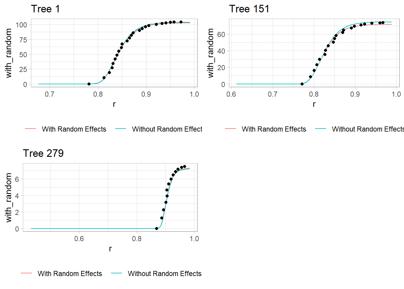
Figure 9.9: Individual Tree Scatter Plot
Red Line: Model predictions with tree-specific random effects.
Teal Line: Model predictions based only on fixed effects (ignoring tree-specific variation).
Dots: Observed cumulative volume for each tree.