10.9 Wavelet Regression
Wavelet regression is a nonparametric regression technique that represents the target function as a combination of wavelet basis functions. Unlike traditional basis functions (e.g., polynomials or splines), wavelets have excellent localization properties in both the time (or space) and frequency domains. This makes wavelet regression particularly effective for capturing local features, such as sharp changes, discontinuities, and transient patterns.
A wavelet is a function \(\psi(t)\) that oscillates (like a wave) but is localized in both time and frequency. The key idea is to represent a function as a linear combination of shifted and scaled versions of a mother wavelet \(\psi(t)\).
Wavelet basis functions are generated by scaling and translating the mother wavelet:
\[ \psi_{j,k}(t) = 2^{j/2} \psi(2^j t - k), \]
where:
- \(j\) (scale parameter): Controls the frequency—larger \(j\) captures finer details (high-frequency components).
- \(k\) (translation parameter): Controls the location—shifting the wavelet along the time or space axis.
- The factor \(2^{j/2}\) ensures that the wavelet basis functions are orthonormal.
In addition to the mother wavelet \(\psi(t)\), there’s also a scaling function \(\phi(t)\), which captures the low-frequency (smooth) components of the data.
10.9.1 Wavelet Series Expansion
Just as Fourier analysis represents functions as sums of sines and cosines, wavelet analysis represents a function as a sum of wavelet basis functions:
\[ f(t) = \sum_{k} c_{J_0, k} \phi_{J_0, k}(t) + \sum_{j = J_0}^{J_{\max}} \sum_{k} d_{j, k} \psi_{j, k}(t), \]
where:
- \(c_{J_0, k}\) are the approximation coefficients at the coarsest scale \(J_0\), capturing smooth trends,
- \(d_{j, k}\) are the detail coefficients at scale \(j\), capturing finer details,
- \(\phi_{J_0, k}(t)\) are the scaling functions, and \(\psi_{j, k}(t)\) are the wavelet functions.
The goal of wavelet regression is to estimate these coefficients based on observed data.
10.9.2 Wavelet Regression Model
Given data \(\{(x_i, y_i)\}_{i=1}^n\), the wavelet regression model assumes:
\[ y_i = f(x_i) + \varepsilon_i, \]
where:
- \(f(x)\) is the unknown regression function,
- \(\varepsilon_i\) are i.i.d. errors with mean zero and variance \(\sigma^2\).
We approximate \(f(x)\) using a finite number of wavelet basis functions:
\[ \hat{f}(x) = \sum_{k} \hat{c}_{J_0, k} \phi_{J_0, k}(x) + \sum_{j = J_0}^{J_{\max}} \sum_{k} \hat{d}_{j, k} \psi_{j, k}(x), \]
where the coefficients \(\hat{c}_{J_0, k}\) and \(\hat{d}_{j, k}\) are estimated from the data.
Coefficient Estimation:
- Linear Wavelet Regression: Estimate coefficients via least squares, projecting the data onto the wavelet basis.
- Nonlinear Wavelet Regression (Thresholding): Apply shrinkage or thresholding (e.g., hard or soft thresholding) to the detail coefficients \(d_{j, k}\) to reduce noise and prevent overfitting. This is especially useful when the true signal is sparse in the wavelet domain.
10.9.3 Wavelet Shrinkage and Thresholding
Wavelet shrinkage is a powerful denoising technique introduced by Donoho and Johnstone (1995). The idea is to suppress small coefficients (likely to be noise) while retaining large coefficients (likely to contain the true signal).
Thresholding Rules:
- Hard Thresholding:
\[ \hat{d}_{j, k}^{\text{(hard)}} = \begin{cases} d_{j, k}, & \text{if } |d_{j, k}| > \tau, \\ 0, & \text{otherwise}, \end{cases} \]
- Soft Thresholding:
\[ \hat{d}_{j, k}^{\text{(soft)}} = \operatorname{sign}(d_{j, k}) \cdot \max\left(|d_{j, k}| - \tau, 0\right), \]
where \(\tau\) is the threshold parameter, often chosen based on the noise level (e.g., via cross-validation or universal thresholding).
| Aspect | Kernel/Local Polynomial | Splines | Wavelets |
|---|---|---|---|
| Smoothness | Smooth, localized | Globally smooth with knots | Captures sharp discontinuities |
| Basis Functions | Kernel functions | Piecewise polynomials | Compact, oscillatory wavelets |
| Handling of Noise | Prone to overfitting without smoothing | Controlled via penalties | Excellent via thresholding |
| Computational Cost | Moderate | High (for large knots) | Efficient (fast wavelet transform) |
| Applications | Curve fitting, density estimation | Smoothing trends | Signal processing, time series |
# Simulated data: Noisy signal with discontinuities
set.seed(123)
n <- 96
x <- seq(0, 1, length.out = n)
signal <-
    sin(4 * pi * x) + ifelse(x > 0.5, 1, 0)  # Discontinuity at x = 0.5
y <- signal + rnorm(n, sd = 0.2)

# Wavelet Regression using Discrete Wavelet Transform (DWT)
library(waveslim)

# Apply DWT with the correct parameter name
dwt_result <- dwt(y, wf = "haar", n.levels = 4)

# Thresholding (currently hard thresholding)
threshold <- 0.2
dwt_result_thresh <- dwt_result
for (i in 1:4) {
    dwt_result_thresh[[i]] <-
        ifelse(abs(dwt_result[[i]]) > threshold, dwt_result[[i]], 0)
}

# for soft thresholding
# for (i in 1:4) {
#     dwt_result_thresh[[i]] <-
#         sign(dwt_result[[i]]) * pmax(abs(dwt_result[[i]]) - threshold, 0)
# }


# Inverse DWT to reconstruct the signal
y_hat <- idwt(dwt_result_thresh)
# Plotting
plot(
x,
y,
type = "l",
col = "gray",
lwd = 1,
main = "Wavelet Regression (Denoising)"
)
lines(x,
signal,
col = "blue",
lwd = 2,
lty = 2) # True signal
lines(x, y_hat, col = "red", lwd = 2) # Denoised estimate
legend(
"topright",
legend = c("Noisy Data", "True Signal", "Wavelet Estimate"),
col = c("gray", "blue", "red"),
lty = c(1, 2, 1),
lwd = c(1, 2, 2)
)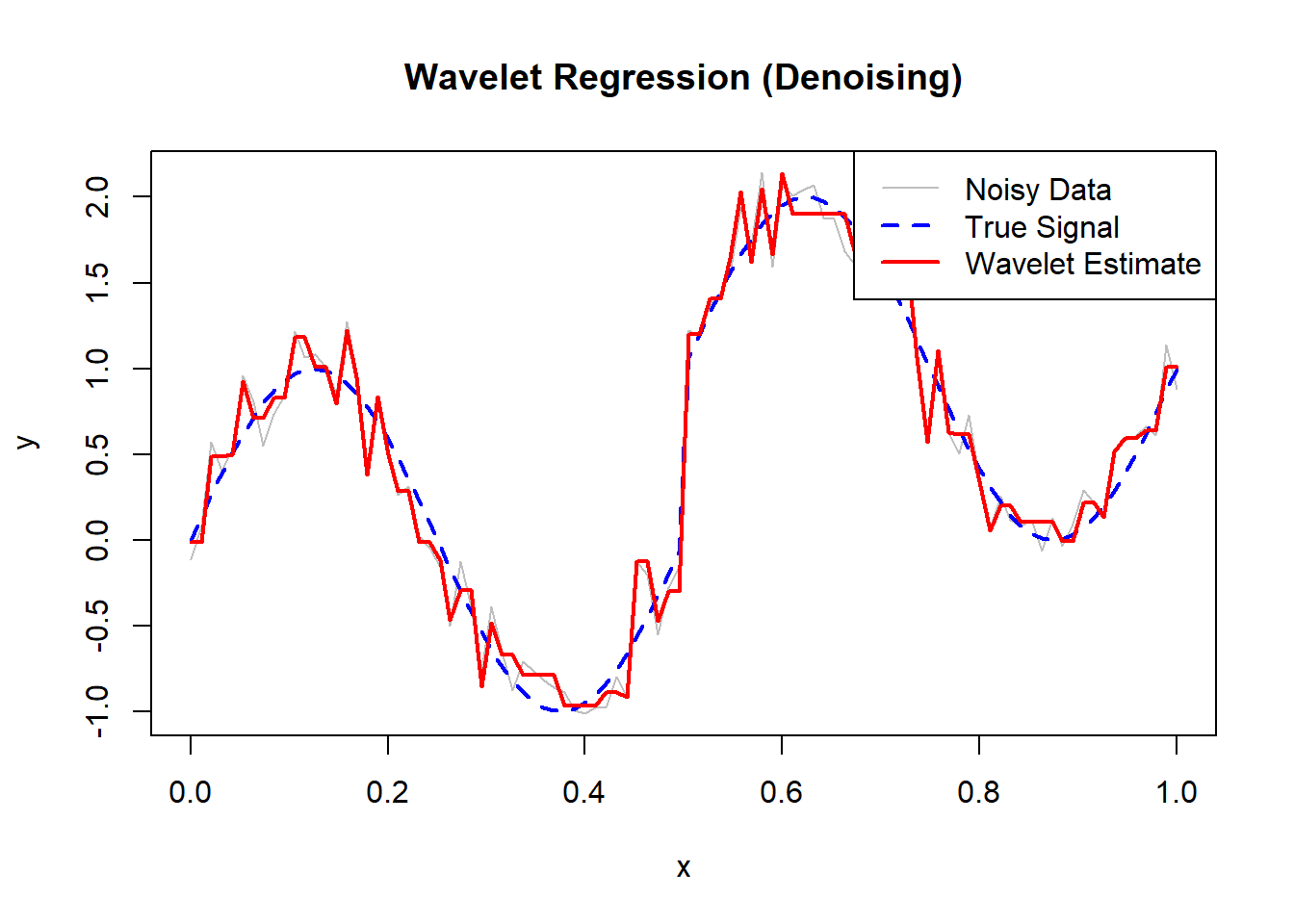
Figure 10.22: Wavelet Regression (Denoising)
Advantages:
Local Feature Detection: Excellent for capturing sharp changes, discontinuities, and localized phenomena.
Multiresolution Analysis: Analyzes data at multiple scales, making it effective for both global trends and fine details.
Denoising Capability: Powerful noise reduction through thresholding in the wavelet domain.
Limitations:
Complexity: Requires careful selection of wavelet basis, decomposition levels, and thresholding methods.
Less Interpretability: Coefficients are less interpretable compared to spline or tree-based methods.
Boundary Effects: May suffer from artifacts near data boundaries without proper treatment.
# Load necessary libraries
library(waveslim)   # For Discrete Wavelet Transform (DWT)
library(ggplot2)


# Simulate Data: Noisy signal with discontinuities
set.seed(123)
n <- 96
x <- seq(0, 1, length.out = n)

# True signal: Sinusoidal with a discontinuity at x = 0.5
signal <- sin(4 * pi * x) + ifelse(x > 0.5, 1, 0)

# Add Gaussian noise
y <- signal + rnorm(n, sd = 0.2)
# Plot the noisy data and true signal
ggplot() +
geom_line(aes(x, y),
color = "gray",
size = 0.8,
alpha = 0.7) +
geom_line(
aes(x, signal),
color = "blue",
linetype = "dashed",
size = 1
) +
labs(title = "Noisy Data with Underlying True Signal",
x = "x", y = "Signal") +
theme_minimal()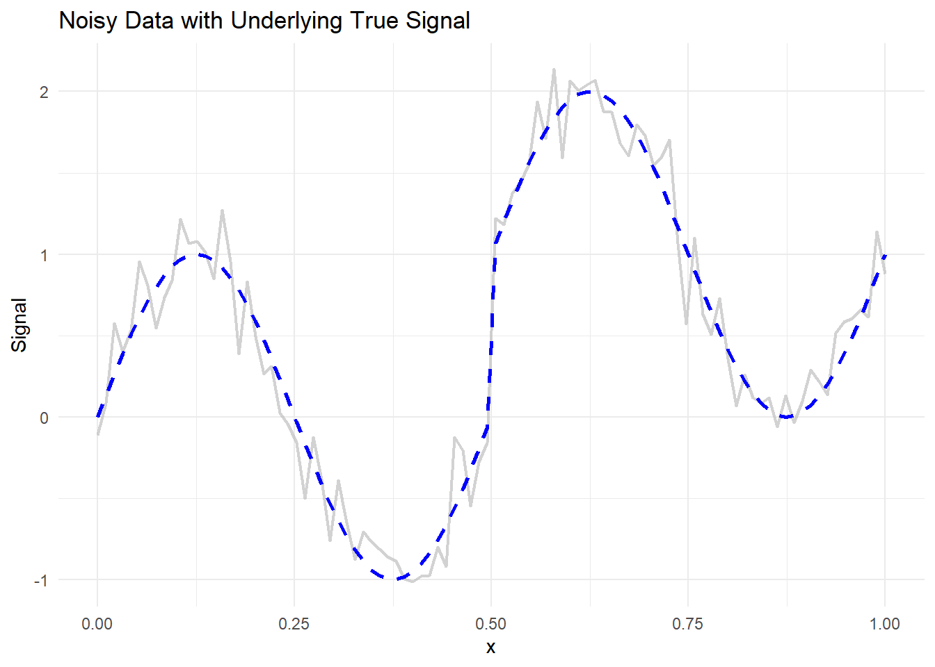
Figure 10.23: Noisy Data with Underlying True Signal
# Apply Discrete Wavelet Transform (DWT) using Haar wavelet
dwt_result <- dwt(y, wf = "haar", n.levels = 4)

# View DWT structure
str(dwt_result)
#> List of 5
#>  $ d1: num [1:48] 0.14 -0.1221 0.3017 -0.1831 0.0745 ...
#>  $ d2: num [1:24] 0.50003 -0.06828 0.35298 0.01582 -0.00853 ...
#>  $ d3: num [1:12] 0.669 0.128 -0.746 -0.532 -0.258 ...
#>  $ d4: num [1:6] 1.07 -1.766 0.752 0.663 -1.963 ...
#>  $ s4: num [1:6] 2.963 -0.159 -2.758 6.945 3.845 ...
#>  - attr(*, "class")= chr "dwt"
#>  - attr(*, "wavelet")= chr "haar"
#>  - attr(*, "boundary")= chr "periodic"
wf = "haar": Haar wavelet, simple and effective for detecting discontinuities.n.levels = 4: Number of decomposition levels (captures details at different scales).
The DWT output contains approximation coefficients and detail coefficients for each level.
# Hard Thresholding
threshold <- 0.2  # Chosen threshold for demonstration
dwt_hard_thresh <- dwt_result

# Apply hard thresholding to detail coefficients
for (i in 1:4) {
  dwt_hard_thresh[[i]] <- ifelse(abs(dwt_result[[i]]) > threshold, dwt_result[[i]], 0)
}
# Soft Thresholding
dwt_soft_thresh <- dwt_result
# Apply soft thresholding to detail coefficients
for (i in 1:4) {
dwt_soft_thresh[[i]] <- sign(dwt_result[[i]]) * pmax(abs(dwt_result[[i]]) - threshold, 0)
}- Hard Thresholding: Keeps coefficients above the threshold, sets others to zero.
- Soft Thresholding: Shrinks coefficients toward zero, reducing potential noise smoothly.
# Reconstruct the denoised signals using Inverse DWT
y_hat_hard <- idwt(dwt_hard_thresh)
y_hat_soft <- idwt(dwt_soft_thresh)
# Combine data for ggplot
df_plot <- data.frame(
x = rep(x, 4),
y = c(y, signal, y_hat_hard, y_hat_soft),
Type = rep(
c(
"Noisy Data",
"True Signal",
"Hard Thresholding",
"Soft Thresholding"
),
each = n
)
)# Plotting
ggplot(df_plot, aes(x, y, color = Type, linetype = Type)) +
geom_line(size = 1) +
scale_color_manual(values = c("gray", "blue", "red", "green")) +
scale_linetype_manual(values = c("solid", "dashed", "solid", "solid")) +
labs(
title = "Wavelet Regression (Denoising)",
subtitle = "Comparison of Hard vs. Soft Thresholding",
x = "x",
y = "Signal"
) +
theme_minimal() +
theme(legend.position = "top")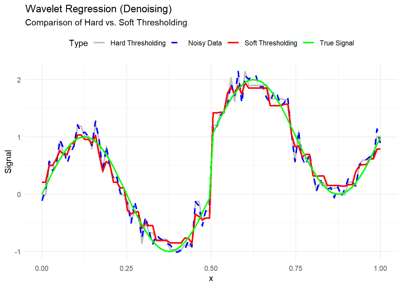
Figure 10.24: Wavelet Regression (Denoising)
# Compute Mean Squared Error (MSE) for each method
mse_noisy <- mean((y - signal) ^ 2)
mse_hard <- mean((y_hat_hard - signal) ^ 2)
mse_soft <- mean((y_hat_soft - signal) ^ 2)

# Display MSE comparison
data.frame(
  Method = c("Noisy Data", "Hard Thresholding", "Soft Thresholding"),
  MSE = c(mse_noisy, mse_hard, mse_soft)
)
#>              Method        MSE
#> 1        Noisy Data 0.03127707
#> 2 Hard Thresholding 0.02814465
#> 3 Soft Thresholding 0.02267171- Lower MSE indicates better denoising performance.
- Soft thresholding often achieves smoother results with lower MSE.