26.5 Assumptions for Identifying Treatment Effects
To identify causal effects in non-randomized studies, we typically rely on three key assumptions:
- Stable Unit Treatment Value Assumption (SUTVA)
- Conditional Ignorability (Unconfoundedness) Assumption
- Overlap (Positivity) Assumption
These assumptions ensure that we can properly define and estimate causal effects, mitigating biases from confounders or selection effects.
26.5.1 Stable Unit Treatment Value Assumption
SUTVA consists of two key components:
- Consistency Assumption: The treatment indicator \(Z \in \{0,1\}\) adequately represents all versions of the treatment.
- No Interference Assumption: A subject’s outcome depends only on its own treatment status and is not affected by the treatment assignments of other subjects.
This assumption ensures that potential outcomes are well-defined and independent of external influences, forming the foundation of Rubin’s Causal Model (RCM). Violations of SUTVA can lead to biased estimators and incorrect standard errors.
Let \(Y_i(Z)\) denote the potential outcome for unit \(i\) under treatment assignment \(Z\), where \(Z \in \{0,1\}\) represents a binary treatment.
SUTVA states that:
\[ Y_i(Z) = Y_i(Z, \mathbf{Z}_{-i}) \]
where \(\mathbf{Z}_{-i}\) denotes the treatment assignments of all other units except \(i\). If SUTVA holds, then:
\[ Y_i(Z) = Y_i(Z, \mathbf{Z}_{-i}) \quad \forall \mathbf{Z}_{-i}. \]
This implies that unit \(i\)’s outcome depends only on its own treatment status and is unaffected by the treatment of others.
26.5.1.1 Implications of SUTVA
If SUTVA holds, the Average Treatment Effect is well-defined as:
\[ \text{ATE} = \mathbb{E}[Y_i(1)] - \mathbb{E}[Y_i(0)]. \]
However, if SUTVA is violated, standard causal inference methods may fail. Common violations include:
- Interference (Spillover Effects): The treatment of one unit influences another’s outcome.
- Example: A marketing campaign for a product influences both treated and untreated customers through word-of-mouth effects.
- Solution: Use spatial econometrics or network-based causal inference models to account for spillovers.
- Treatment Inconsistency: Multiple versions of a treatment exist but are not explicitly modeled.
- Example: Different incentive levels in a sales promotion may have different effects.
- Solution: Explicitly define and distinguish different treatment versions using principal stratification.
Violating SUTVA introduces significant challenges in causal inference (Table 26.3)
| Issue | Consequence |
| Bias in Estimators | If interference is ignored, treatment effects may be over- or underestimated. |
| Incorrect Standard Errors | Standard errors may be underestimated (if spillovers are ignored) or overestimated (if hidden treatment variations exist). |
| Ill-Defined Causal Effects | If multiple treatment versions exist, it becomes unclear which causal effect is being estimated. |
Thus, when SUTVA is unlikely to hold, researchers must adopt more flexible methodologies to ensure valid inferences.
26.5.1.2 No Interference
The no interference component of the Stable Unit Treatment Value Assumption states that one unit’s treatment assignment does not influence another unit’s outcome. However, in many real-world scenarios, this assumption is violated due to spillover effects, such as:
- Epidemiology: In vaccine studies, an individual’s health status may depend on the vaccination status of their social network.
- Marketing Experiments: In online advertising, one consumer’s exposure to an ad campaign may influence their peers’ purchasing behavior.
From an economist’s point of view, this “no interference” condition quickly morphs into a list of assumptions about market isolation, absence of spillovers, and partial equilibrium thinking.
Mathematically, let \(Y_i(\mathbf{Z})\) be the potential outcome for unit \(i\) given treatment assignments \(\mathbf{Z} = (Z_1, \dots, Z_N)\) for all units. No interference means:
\[ Y_i(\mathbf{Z}) = Y_i(Z_i) \]
That is, unit \(i\)’s outcome depends only on its own treatment \(Z_i\), not on \(Z_j\) for \(j \neq i\).
Alternatively, we can write interference occurs when unit \(i\)’s outcome depends on the treatment assignments of other units within a neighborhood function \(\mathcal{N}(i)\):
\[ Y_i(Z_i, \mathbf{Z}_{\mathcal{N}(i)}), \]
where \(\mathbf{Z}_{\mathcal{N}(i)}\) represents the treatment assignments of neighboring units. If \(\mathcal{N}(i) \neq \emptyset\), then SUTVA is violated, necessitating alternative modeling approaches such as spatial econometrics, network-based causal inference, or graph-based treatment effect estimation.
Special Cases of Interference
Several forms of interference can arise in applied settings:
- Complete Interference: Each unit’s outcome depends on the treatment assignments of all other units (e.g., in a fully connected social network).
- Partial Interference: Interference occurs within subgroups but not between them (e.g., students within classrooms but not across schools).
- Network Interference: Treatment effects propagate through a social or spatial network, requiring models such as graph-based causal inference or spatial econometrics.
Each of these cases necessitates adjustments to standard causal inference techniques.
Economists hear “no interference” and think:
- “No externalities”
- “No peer effects”
- “Partial equilibrium”
- “Small shock in a big market”
- “No strategic interaction”
Table 26.4 maps the statistical and economic language.
| Statistical Term | Economic Translation | Economic Intuition |
|---|---|---|
| No interference between units | No externalities | My treatment does not affect your utility or production function |
| Outcomes depend only on own treatment | No peer effects | My grade is unaffected by whether my classmates are treated |
| Unit’s treatment does not affect prices | Partial equilibrium | Market prices remain fixed regardless of who is treated |
| Treated unit is infinitesimal | No general equilibrium feedback | Treated fraction too small to shift aggregate supply/demand |
| No network dependence | No spillovers | No migration, contagion, or supply-chain effects to others |
In many economic settings, no interference is a very strong assumption because:
- Markets are connected: Price changes in one market can propagate to others.
- Agents are strategic: Competitors, consumers, or workers adjust behavior in response to others’ treatment.
- Resources are scarce: Treatments may affect availability of goods, labor, or credit elsewhere.
- Networks matter: Information, contagion, or migration can link outcomes.
Economists often default to a partial equilibrium view to approximate no interference: analyze a small slice of the market where general equilibrium effects are negligible (Table 26.5).
| Scenario | Why Interference Occurs | Type of Spillover |
|---|---|---|
| Housing voucher experiment | Treated households bid up rents in the same area | Price-mediated spillover |
| Tax break to one industry | Shifts labor and capital into that industry, affecting others | Factor market reallocation |
| Vaccination program | Reduces disease prevalence for all | Epidemiological spillover |
| New export subsidy | Alters exchange rate, affecting other exporters | Macroeconomic spillover |
When No Interference is Plausible
- The treatment is randomized at a micro level and only a tiny fraction of units are treated.
- Units are geographically, socially, and economically isolated.
- Outcomes are determined before any interaction could occur.
- Institutional separation ensures one unit’s treatment cannot affect another (e.g., sealed laboratory experiments).
Key takeaway: Statisticians define no interference narrowly: my potential outcomes depend only on my own treatment. Economists translate this into a battery of market-isolation assumptions, usually under a partial equilibrium frame. In most economic applications, the challenge is not assuming no interference, but modeling and estimating the ways in which it is violated.
26.5.1.4 Strategies to Address SUTVA Violations
Several approaches help mitigate the effects of SUTVA violations:
- Randomized Saturation Designs: Assign treatment at varying intensities across clusters to estimate spillover effects.
- Network-Based Causal Models: Utilize graph theory or adjacency matrices to account for interference.
- Instrumental Variables: If multiple versions of a treatment exist, use an IV to isolate a single version.
- Stratified Analysis: When treatment variations are known, analyze subgroups separately.
- Difference-in-Differences with Spatial Controls: Incorporate spatial lag terms to model geographic spillovers.
26.5.2 Conditional Ignorability Assumption
Next, we must assume that treatment assignment is independent of the potential outcomes conditional on the observed covariates. This assumption has several equivalent names in the causal inference literature, including
Conditional Ignorability
Conditional Exchangeability
No Unobserved Confounding
No Omitted Variables
In the language of causal diagrams, this assumption ensures that all backdoor paths between treatment and outcome are blocked by observed covariates.
Formally, we assume that treatment assignment \(Z\) is independent of the potential outcomes \(Y(Z)\) given a set of observed covariates \(X\):
\[ Y(1), Y(0) \perp\!\!\!\perp Z \mid X. \]
This means that after conditioning on \(X\), the probability of receiving treatment is unrelated to the potential outcomes, ensuring that comparisons between treated and untreated units are unbiased.
In causal inference, treatment assignment is said to be ignorable if, conditional on observed covariates \(X\), the treatment indicator \(Z\) is independent of the potential outcomes:
\[ P(Y(1), Y(0) \mid Z, X) = P(Y(1), Y(0) \mid X). \]
Equivalently, in terms of conditional probability:
\[ P(Z = 1 \mid Y(1), Y(0), X) = P(Z = 1 \mid X). \]
This ensures that treatment assignment is as good as random once we control for \(X\), meaning that the probability of receiving treatment does not depend on unmeasured confounders.
A direct consequence is that we can estimate the Average Treatment Effect using observational data:
\[ \mathbb{E}[Y(1) - Y(0)] = \mathbb{E}[\mathbb{E}[Y \mid Z=1, X] - \mathbb{E}[Y \mid Z=0, X]]. \]
If ignorability holds, standard regression models, matching, or weighting techniques (e.g., propensity score weighting) can provide unbiased causal estimates.
26.5.2.1 The Role of Causal Diagrams and Backdoor Paths
In causal diagrams (DAGs), confounding arises when a backdoor path exists between treatment \(Z\) and outcome \(Y\). A backdoor path is any non-causal path that creates spurious associations between \(Z\) and \(Y\). The conditional ignorability assumption requires that all such paths be blocked by conditioning on a sufficient set of covariates \(X\).
Consider a simple causal diagram in Figure 26.1.
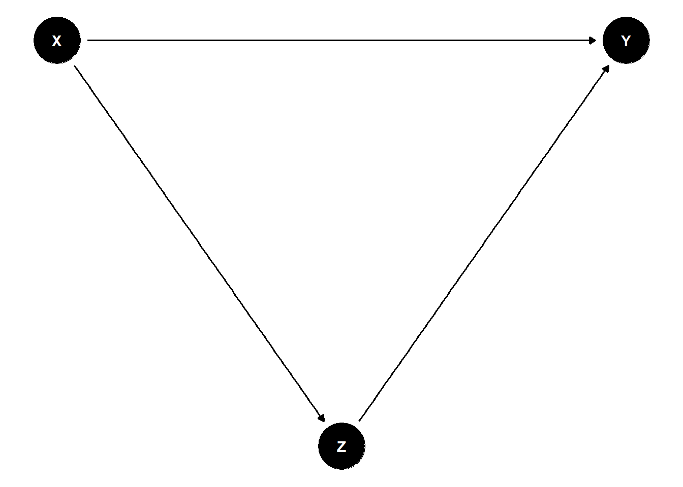
Figure 26.1: Directed Acyclic Graph
Here, \(X\) is a common cause of both \(Z\) and \(Y\), creating a backdoor path \(Z \leftarrow X \rightarrow Y\). If we fail to control for \(X\), the estimated effect of \(Z\) on \(Y\) will be biased. However, if we condition on \(X\), we block the backdoor path and obtain an unbiased estimate of the treatment effect.
To satisfy the conditional ignorability assumption, researchers must identify a sufficient set of confounders to block all backdoor paths. This is often done using domain knowledge and causal structure learning algorithms.
- Minimal Sufficient Adjustment Set: The smallest set of covariates \(X\) that, when conditioned upon, satisfies ignorability.
- Propensity Score Methods: Instead of adjusting directly for \(X\), one can estimate the probability of treatment \(P(Z=1 \mid X)\) and use inverse probability weighting or matching.
26.5.2.2 Violations of the Ignorability Assumption
If ignorability does not hold, treatment assignment depends on unobserved confounders, introducing omitted variable bias. Mathematically, if there exists an unmeasured variable \(U\) such that:
\[ Y(1), Y(0) \not\perp\!\!\!\perp Z \mid X, \]
then estimates of the treatment effect will be biased.
Consequences of Violations
- Confounded Estimates: The estimated treatment effect captures both the causal effect and the bias from unobserved confounders.
- Selection Bias: If treatment assignment is related to factors that also influence the outcome, the sample may not be representative.
- Overestimation or Underestimation: Ignoring important confounders can lead to inflated or deflated estimates of treatment effects.
Example of Confounding
Consider an observational study on smoking and lung cancer (Figure 26.2).
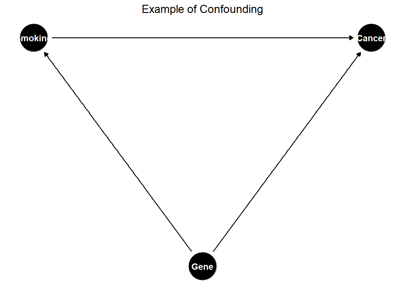
Figure 26.2: Example of Confounding in a Causal Diagram
Here, genetics is an unmeasured confounder affecting both smoking and lung cancer. If we do not control for genetics, the estimated effect of smoking on lung cancer will be biased.
26.5.2.3 Strategies to Address Violations
If ignorability is violated due to unobserved confounding, several techniques can be used to mitigate bias:
- Instrumental Variables:
- Use a variable \(W\) that affects treatment \(Z\) but has no direct effect on \(Y\), ensuring exogeneity.
- Example: Randomized incentives to encourage treatment uptake.
- Difference-in-Differences:
- Compare changes in outcomes before and after treatment in a treated vs. control group.
- Requires a parallel trends assumption.
- Regression Discontinuity:
- Exploit cutoff-based treatment assignment.
- Example: Scholarship eligibility at a certain GPA threshold.
- Propensity Score Methods:
- Estimate the probability of treatment given \(X\).
- Use matching, inverse probability weighting (IPW), or stratification to balance treatment groups.
- Sensitivity Analysis:
- Quantify how much unobserved confounding would be needed to alter conclusions.
- Example: Rosenbaum’s sensitivity bounds.
26.5.2.4 Practical Considerations
How to Select Covariates \(X\)?
- Domain Knowledge: Consult experts to identify potential confounders.
- Causal Discovery Methods: Use Bayesian networks or structure learning to infer relationships.
- Statistical Tests: Examine balance in pre-treatment characteristics.
Trade-Offs in Covariate Selection
- Too Few Covariates → Risk of omitted variable bias.
- Too Many Covariates → Overfitting, loss of efficiency in estimation.
26.5.3 Overlap (Positivity) Assumption
The overlap assumption, also known as common support or positivity, ensures that the probability of receiving treatment is strictly between 0 and 1 for all values of the observed covariates \(X_i\). Mathematically, this is expressed as:
\[ 0 < P(Z_i = 1 \mid X_i) < 1, \quad \forall X_i. \]
This condition ensures that for every possible value of \(X_i\), there is a nonzero probability of receiving both treatment (\(Z_i = 1\)) and control (\(Z_i = 0\)). That is, the covariate distributions of treated and control units must overlap.
When overlap is limited, the Average Treatment Effect may not be identifiable. In some cases, the Average Treatment Effect on the Treated remains identifiable, but extreme violations of overlap can make even ATT estimation problematic. An alternative estimand, the Average Treatment Effect for the Overlap Population (ATO), may be used instead, focusing on a subpopulation where treatment assignment is not deterministic (F. Li, Morgan, and Zaslavsky 2018).
While the ATO offers a practical solution in the presence of limited overlap, researchers may still prefer more conventional estimands like the ATT for interpretability and policy relevance. In such cases, balancing weights present a valuable alternative to inverse probability weights. Unlike Inverse Probability Weighting, which can yield extreme weights under poor overlap, balancing weights directly address covariate imbalance during the estimation process. Ben-Michael and Keele (2023) demonstrate that balancing weights can recover the ATT even when inverse probability weighting fails due to limited overlap. Although overlap weights remain an important tool for reducing bias, balancing weights enable researchers to target familiar causal estimands like the ATT, offering a compelling compromise between statistical robustness and interpretability.
The overlap assumption prevents cases where treatment assignment is deterministic, ensuring that:
\[ 0 < P(Z_i = 1 \mid X_i) < 1, \quad \forall X_i. \]
This implies two key properties:
- Positivity Condition: Every unit has a nonzero probability of receiving treatment.
- No Deterministic Treatment Assignment: If \(P(Z_i = 1 \mid X_i) = 0\) or \(P(Z_i = 1 \mid X_i) = 1\) for some \(X_i\), then the causal effect is not identifiable for those values.
If some subpopulations always receive treatment (\(P(Z_i = 1 \mid X_i) = 1\)) or never receive treatment (\(P(Z_i = 1 \mid X_i) = 0\)), then there is no counterfactual available, making causal inference impossible for those groups.
26.5.3.1 Implications of Violating the Overlap Assumption
When the overlap assumption is violated, identifying causal effects becomes challenging (Table 26.6).
| Issue | Consequence |
|---|---|
| Limited Generalizability of ATE | ATE cannot be estimated if there is poor overlap in covariate distributions. |
| ATT May Still Be Identifiable | ATT can be estimated if some overlap exists, but it is restricted to the treated group. |
| Severe Violations Can Prevent ATT Estimation | If there is no overlap, even ATT is not identifiable. |
| Extrapolation Bias | Weak overlap forces models to extrapolate, leading to unstable and biased estimates. |
Example: Education Intervention and Socioeconomic Status
Suppose we study an education intervention aimed at improving student performance. If only high-income students received the intervention (\(P(Z = 1 \mid X) = 1\) for high income) and no low-income students received it (\(P(Z = 1 \mid X) = 0\) for low income), then there is no common support. As a result, we cannot estimate a valid treatment effect for low-income students.
26.5.3.2 Diagnosing Overlap Violations
Before estimating causal effects, it is crucial to assess overlap using diagnostic tools such as:
- Propensity Score Distribution
Estimate the propensity score \(e(X) = P(Z = 1 \mid X)\) and visualize its distribution:
- Good Overlap (Well-Mixed Propensity Score Distributions) → Treated and control groups have similar propensity score distributions.
- Poor Overlap (Separated Propensity Score Distributions) → Clear separation in propensity score distributions suggests limited common support.
- Standardized Mean Differences
Compare covariate distributions between treated and control groups. Large imbalances suggest weak overlap.
- Kernel Density Plots
Visualize the density of propensity scores in each treatment group. Non-overlapping regions indicate poor support.
26.5.3.3 Strategies to Address Overlap Violations
If overlap is weak, several strategies can help:
- Trimming Non-Overlapping Units
- Exclude units with extreme propensity scores (e.g., \(P(Z = 1 \mid X) \approx 0\) or \(P(Z = 1 \mid X) \approx 1\)).
- Improves internal validity but reduces sample size.
- Reweighting Approaches
- Use overlap weights to focus on a population where treatment was plausibly assignable.
- The Average Treatment Effect for the Overlap Population (ATO) estimates effects for units where \(P(Z = 1 \mid X)\) is moderate (e.g., close to 0.5).
- Matching on the Propensity Score
- Remove units that lack suitable matches in the opposite treatment group.
- Improves balance at the cost of excluding observations.
- Covariate Balancing Techniques
- Use entropy balancing or inverse probability weighting to adjust for limited overlap.
- Sensitivity Analysis
- Assess how overlap violations affect causal conclusions.
- Example: Rosenbaum’s sensitivity bounds quantify the impact of unmeasured confounding.
26.5.3.4 Average Treatment Effect for the Overlap Population
When overlap is weak, ATO offers an alternative estimand that focuses on the subpopulation where treatment is not deterministic.
Instead of estimating the ATE (which applies to the entire population) or the ATT (which applies to the treated population), ATO focuses on units where both treatment and control were plausible options (Table 26.7).
ATO is estimated using overlap weights:
\[ W_i = P(Z_i = 1 \mid X_i) (1 - P(Z_i = 1 \mid X_i)). \]
These weights:
- Downweight extreme propensity scores (where \(P(Z = 1 \mid X)\) is close to 0 or 1).
- Focus inference on the subpopulation with the most overlap.
- Improve robustness in cases with limited common support.
| Estimand | Target Population | Overlap Requirement |
|---|---|---|
| ATE | Entire population | Strong |
| ATT | Treated population | Moderate |
| ATO | Overlap population | Weak |
Practical Applications of ATO
- Policy Evaluation: When treatment assignment is highly structured, ATO ensures conclusions are relevant to a feasible intervention group.
- Observational Studies: Avoids extrapolation bias when estimating treatment effects in subpopulations with common support.