10.5 Smoothing Splines

A spline is a piecewise polynomial function that is smooth at the junction points (called knots). Smoothing splines provide a flexible nonparametric regression technique by balancing the trade-off between closely fitting the data and maintaining smoothness. This is achieved through a penalty on the function’s curvature.

In the univariate case, suppose we have data $\{(x_i, y_i)\}_{i=1}^n$ with $0 \le x_1 < x_2 < \cdots < x_n \le 1$ (rescaling is always possible if needed). The smoothing spline estimator $\hat{m}(x)$ is defined as the solution to the following optimization problem:

$$\hat{m}(x) = \underset{f \in \mathcal{H}}{\arg\min} \left\{ \sum_{i=1}^n \left(y_i - f(x_i)\right)^2 + \lambda \int_{0}^{1} \left(f''(t)\right)^2 \, dt \right\},$$

where:

• The first term measures the lack of fit (residual sum of squares).
• The second term is a roughness penalty that discourages excessive curvature in $f$, controlled by the smoothing parameter $\lambda \ge 0$.
• The space $\mathcal{H}$ denotes the set of all twice-differentiable functions on $[0,1]$.

Special Cases:

• When $\lambda = 0$: No penalty is applied, and the solution interpolates the data exactly (an interpolating spline).
• As $\lambda \to \infty$: The penalty dominates, forcing the solution to be as smooth as possible—reducing to a linear regression (since the second derivative of a straight line is zero).

10.5.1 Properties and Form of the Smoothing Spline

A key result from spline theory is that the minimizer $\hat{m}(x)$ is a natural cubic spline with knots at the observed data points $\{x_1, \ldots, x_n\}$. This result holds despite the fact that we are minimizing over an infinite-dimensional space of functions.

The solution can be expressed as:

$$\hat{m}(x) = a_0 + a_1 x + \sum_{j=1}^n b_j \, (x - x_j)_+^3,$$

where:

• $(u)_+ = \max(u, 0)$ is the positive part function (the cubic spline basis function),
• The coefficients $\{a_0, a_1, b_1, \ldots, b_n\}$ are determined by solving a system of linear equations derived from the optimization problem.

This form implies that the spline is a cubic polynomial within each interval between data points, with smooth transitions at the knots. The smoothness conditions ensure continuity of the function and its first and second derivatives at each knot.

10.5.2 Choice of $\lambda$

The smoothing parameter $\lambda$ plays a crucial role in controlling the trade-off between goodness-of-fit and smoothness:

• Large $\lambda$: Imposes a strong penalty on the roughness, leading to a smoother (potentially underfitted) function that captures broad trends.
• Small $\lambda$: Allows the function to closely follow the data, possibly resulting in overfitting if the data are noisy.

A common approach to selecting $\lambda$ is generalized cross-validation (GCV), which provides an efficient approximation to leave-one-out cross-validation:

$$\mathrm{GCV}(\lambda) = \frac{\frac{1}{n} \sum_{i=1}^n \left(y_i - \hat{m}_{\lambda}(x_i)\right)^2}{\left[1 - \frac{\operatorname{tr}(\mathbf{S}_\lambda)}{n}\right]^2},$$

where:

• $\hat{m}_{\lambda}(x_i)$ is the fitted value at $x_i$ for a given $\lambda$,
• $\mathbf{S}_\lambda$ is the smoothing matrix (or influence matrix) such that $\hat{\mathbf{y}} = \mathbf{S}_\lambda \mathbf{y}$,
• $\operatorname{tr}(\mathbf{S}_\lambda)$ is the effective degrees of freedom, reflecting the model’s flexibility.

The optimal $\lambda$ minimizes the GCV score, balancing fit and complexity without the need to refit the model multiple times (as in traditional cross-validation).

---

10.5.3 Connection to Reproducing Kernel Hilbert Spaces

Smoothing splines can be viewed through the lens of reproducing kernel Hilbert spaces (RKHS). The penalty term:

$$\int_{0}^{1} \left(f''(t)\right)^2 \, dt$$

defines a semi-norm that corresponds to the squared norm of $f$ in a particular RKHS associated with the cubic spline kernel. This interpretation reveals that smoothing splines are equivalent to solving a regularization problem in an RKHS, where the penalty controls the smoothness of the solution.

This connection extends naturally to more general kernel-based methods (e.g., Gaussian process regression, kernel ridge regression) and higher-dimensional spline models.

---

# Load necessary libraries
library(ggplot2)
library(gridExtra)

# 1. Simulate Data
set.seed(123)


# Generate predictor x and response y
n <- 100
x <- sort(runif(n, 0, 10))  # Sorted for smoother visualization
true_function <-
    function(x)
        sin(x) + 0.5 * cos(2 * x)  # True regression function
y <-
    true_function(x) + rnorm(n, sd = 0.3) # Add Gaussian noise

# Visualization of the data
ggplot(data.frame(x, y), aes(x, y)) +
    geom_point(color = "darkblue", alpha = 0.6) +
    geom_line(aes(y = true_function(x)),
              color = "red",
              linetype = "dashed") +
    labs(title = "Simulated Data with True Regression Function",
         x = "x", y = "y") +
    theme_minimal()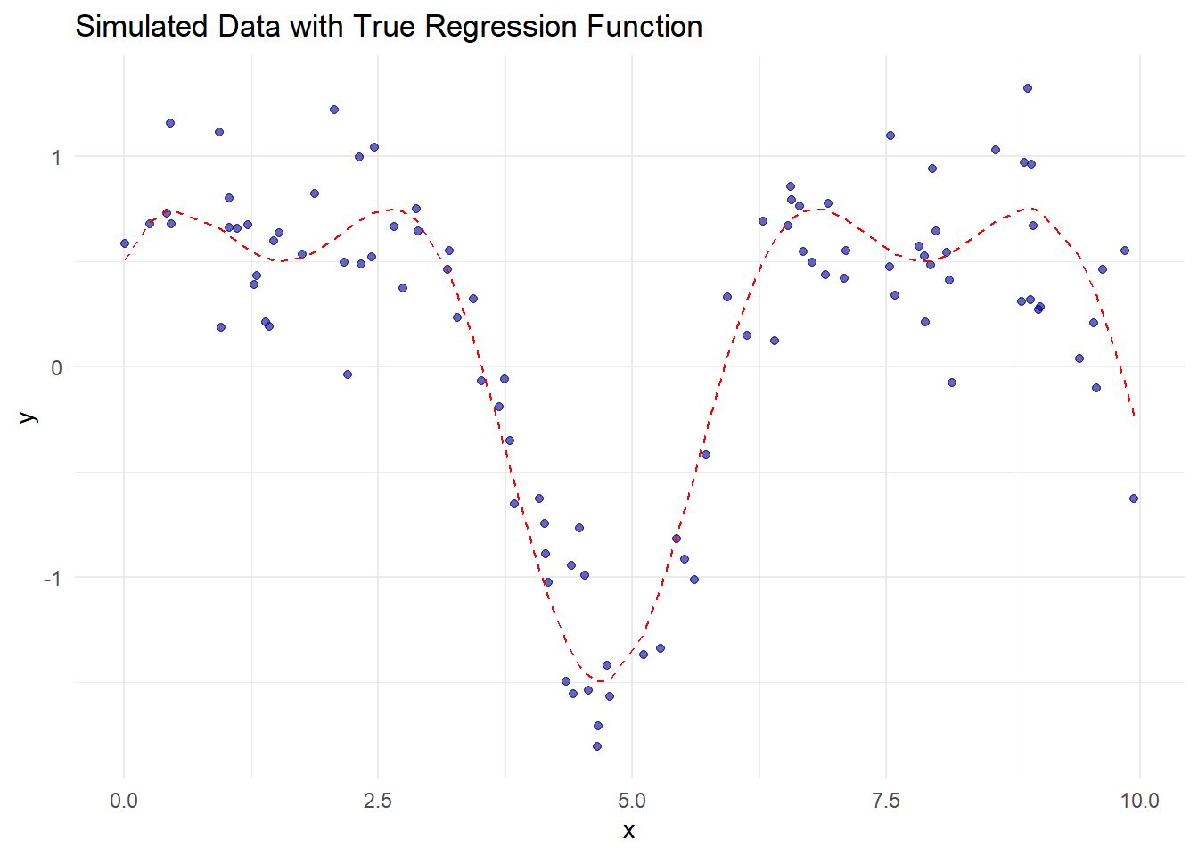

<img src=“10-nonparam-regression_files/figure-html/unnamed-chunk-5-1.png” alt=“Scatter plot titled”Simulated Data with True Regression Function” showing blue data points distributed along the x-axis from 0 to 10 and y-axis from -1 to 1. A red dashed line represents the true regression function, illustrating a non-linear trend with peaks and troughs. The x-axis is labeled “x” and the y-axis is labeled “y”.” width=“90%” />

Figure 2.5: Simulated Data with True Regression Function

# Apply Smoothing Spline with Default Lambda 
# (automatically selected using GCV)
spline_fit_default <- smooth.spline(x, y)

# Apply Smoothing Spline with Manual Lambda 
# (via smoothing parameter 'spar')
spline_fit_smooth <- smooth.spline(x, y, spar = 0.8)  # Smoother fit
spline_fit_flexible <-
    smooth.spline(x, y, spar = 0.4)  # More flexible fit

# Create grid for prediction
x_grid               <- seq(0, 10, length.out = 200)
spline_pred_default  <- predict(spline_fit_default, x_grid)
spline_pred_smooth   <- predict(spline_fit_smooth, x_grid)
spline_pred_flexible <- predict(spline_fit_flexible, x_grid)

# Plot Smoothing Splines with Different Smoothness Levels
ggplot() +
    geom_point(aes(x, y), color = "darkblue", alpha = 0.5) +
    geom_line(aes(x_grid, spline_pred_default$y),
              color = "green",
              size = 1.2) +
    geom_line(
        aes(x_grid, spline_pred_smooth$y),
        color = "orange",
        size = 1.2,
        linetype = "dotted"
    ) +
    geom_line(
        aes(x_grid, spline_pred_flexible$y),
        color = "purple",
        size = 1.2,
        linetype = "dashed"
    ) +
    geom_line(
        aes(x_grid, true_function(x_grid)),
        color = "red",
        linetype = "solid",
        size = 1
    ) +
    labs(
        title = "Smoothing Spline Fits",
        subtitle = "Green: GCV-selected | Orange: Smooth (spar=0.8) | Purple: Flexible (spar=0.4)",
        x = "x",
        y = "Estimated m(x)"
    ) +
    theme_minimal()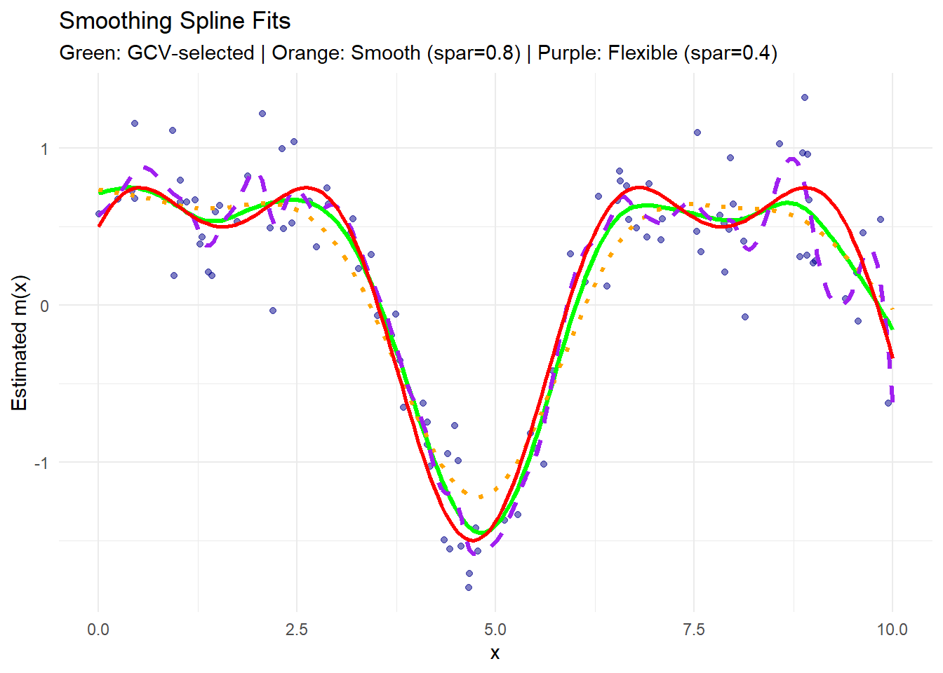

<img src=“10-nonparam-regression_files/figure-html/Visualization of Smoothing Spline Fits-1.png” alt=“Chart titled”Smoothing Spline Fits” showing data points and three smoothing lines. The x-axis is labeled “x” and the y-axis is labeled “Estimated m(x).” The green line represents “GCV-selected,” the orange line is “Smooth (spar=0.8),” and the purple line is “Flexible (spar=0.4).” The chart illustrates how different smoothing parameters affect the fit of the data.” width=“90%” />

(#fig:Visualization of Smoothing Spline Fits)Smoothing Spline Fits

• The green curve is the fit with the optimal $\lambda$ selected automatically via GCV.
• The orange curve (with spar = 0.8) is smoother, capturing broad trends but missing finer details.
• The purple curve (with spar = 0.4) is more flexible, fitting the data closely, potentially overfitting noise.
• The red solid line represents the true regression function.

# Extract Generalized Cross-Validation (GCV) Scores
spline_fit_default$cv.crit  # GCV criterion for the default fit
#> [1] 0.09698728

# Compare GCV for different spar values
spar_values <- seq(0.1, 1.5, by = 0.05)
gcv_scores <- sapply(spar_values, function(spar) {
    fit <- smooth.spline(x, y, spar = spar)
    fit$cv.crit
})

# Optimal spar corresponding to the minimum GCV score
optimal_spar <- spar_values[which.min(gcv_scores)]
optimal_spar
#> [1] 0.7

# GCV Plot
ggplot(data.frame(spar_values, gcv_scores),
       aes(x = spar_values, y = gcv_scores)) +
    geom_line(color = "blue", size = 1) +
    geom_point(aes(x = optimal_spar, y = min(gcv_scores)),
               color = "red",
               size = 3) +
    labs(
        title = "GCV for Smoothing Parameter Selection",
        subtitle = paste("Optimal spar =", round(optimal_spar, 2)),
        x = "Smoothing Parameter (spar)",
        y = "GCV Score"
    ) +
    theme_minimal()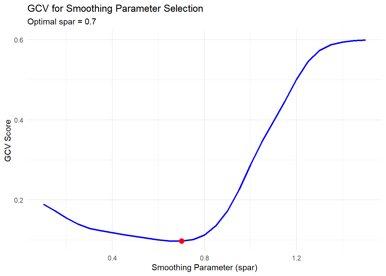

<img src=“10-nonparam-regression_files/figure-html/Plotting GCV Scores-1.png” alt=“Graph titled”GCV for Smoothing Parameter Selection” showing the relationship between the smoothing parameter (spar) on the x-axis and the GCV score on the y-axis. The curve is blue, with a minimum point marked by a red dot at spar = 0.7, indicating the optimal smoothing parameter. The GCV score ranges from 0.2 to 0.6.” width=“90%” />

(#fig:Plotting GCV Scores)GCV for Smoothing Parameter Selection

• The blue curve shows how the GCV score changes with different smoothing parameters (spar).
• The red point indicates the optimal smoothing parameter that minimizes the GCV score.
• Low spar values correspond to flexible fits (risking overfitting), while high spar values produce smoother fits (risking underfitting).

# Apply Smoothing Spline with Optimal spar
spline_fit_optimal <- smooth.spline(x, y, spar = optimal_spar)
spline_pred_optimal <- predict(spline_fit_optimal, x_grid)

# Plot Final Fit
ggplot() +
    geom_point(aes(x, y), color = "gray60", alpha = 0.5) +
    geom_line(aes(x_grid, spline_pred_optimal$y),
              color = "green",
              size = 1.5) +
    geom_line(
        aes(x_grid, true_function(x_grid)),
        color = "red",
        linetype = "dashed",
        size = 1.2
    ) +
    labs(
        title = "Smoothing Spline with Optimal Smoothing Parameter",
        subtitle = paste("Optimal spar =", round(optimal_spar, 2)),
        x = "x",
        y = "Estimated m(x)"
    ) +
    theme_minimal()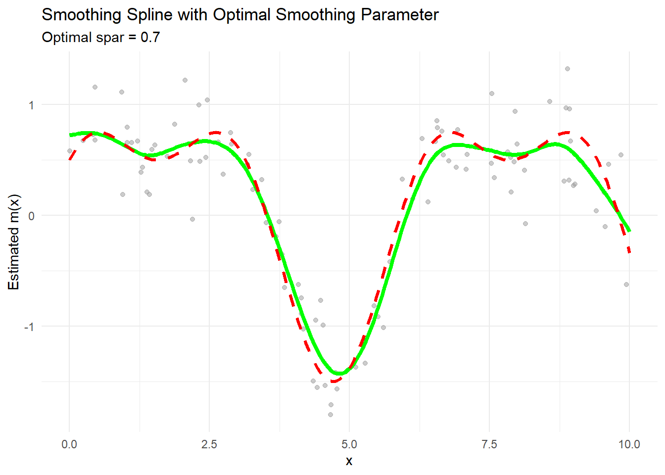

<img src=“10-nonparam-regression_files/figure-html/Final Smoothing Spline Fit with Optimal lambda-1.png” alt=“Scatter plot showing a smoothing spline with an optimal smoothing parameter of 0.7. The x-axis is labeled”x” and the y-axis is labeled “Estimated m(x).” Gray data points are scattered throughout the plot. A green line represents the smoothing spline, with a red dashed line indicating true function.” width=“90%” />

(#fig:Final Smoothing Spline Fit with Optimal lambda)Smoothing Spline with Optimal Smoothing Parameter

---