32.14 Applications
32.14.1 Synthetic Control Estimation
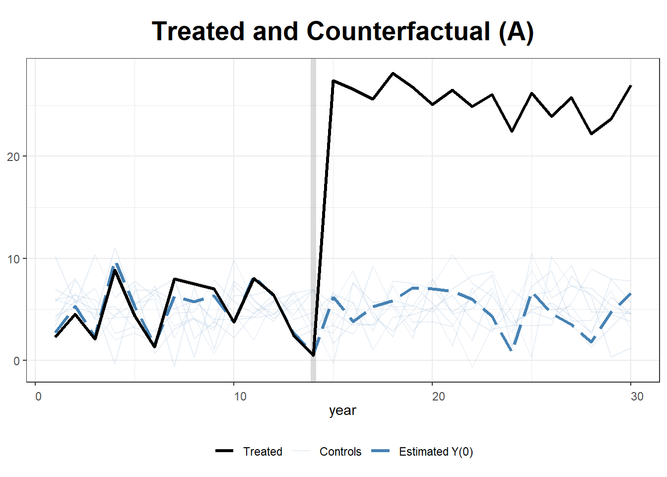
This example simulates data for 10 states over 30 years, where State A receives treatment after year 15. We implement two approaches:
- Standard Synthetic Control using
Synth. - Generalized Synthetic Control using
gsynth, which incorporates iterative fixed effects and multiple treated units.
Load Required Libraries
We construct a panel dataset where the outcome variable \(Y\) is influenced by two covariates (\(X_1, X_2\)). Treatment (\(T\)) is applied to State A from year 15 onwards, with an artificial treatment effect of +20.
# Simulate panel data
set.seed(1)

df <- data.frame(
  year      = rep(1:30, 10),          # 30 years for 10 states
  state     = rep(LETTERS[1:10], each = 30),  # States A to J
  X1        = round(rnorm(300, 2, 1), 2),     # Continuous covariate
  X2        = round(rbinom(300, 1, 0.5) + rnorm(300), 2),  # Binary + noise
  state.num = rep(1:10, each = 30)    # Numeric identifier for states
)

# Outcome variable: Y = 1 + 2 * X1 + noise
df$Y <- round(1 + 2 * df$X1 + rnorm(300), 2)

# Assign treatment: Only State A (state == "A") from year 15 onward
df$T <- as.integer(df$state == "A" & df$year >= 15)

# Apply treatment effect: Increase Y by 20 where treatment is applied
df$Y[df$T == 1] <- df$Y[df$T == 1] + 20

# View data structure
str(df)
#> 'data.frame':    300 obs. of  7 variables:
#>  $ year     : int  1 2 3 4 5 6 7 8 9 10 ...
#>  $ state    : chr  "A" "A" "A" "A" ...
#>  $ X1       : num  1.37 2.18 1.16 3.6 2.33 1.18 2.49 2.74 2.58 1.69 ...
#>  $ X2       : num  1.96 0.4 -0.75 -0.56 -0.45 1.06 0.51 -2.1 0 0.54 ...
#>  $ state.num: int  1 1 1 1 1 1 1 1 1 1 ...
#>  $ Y        : num  2.29 4.51 2.07 8.87 4.37 1.32 8 7.49 6.98 3.72 ...
#>  $ T        : int  0 0 0 0 0 0 0 0 0 0 ...
Step 1: Estimating Synthetic Control with Synth
The Synth package creates a synthetic control by matching pre-treatment trends of the treated unit (State A) with a weighted combination of donor states.
We specify predictors, dependent variable, and donor pool.
dataprep.out <- dataprep(
  df,
  predictors = c("X1", "X2"),
  dependent = "Y",
  unit.variable = "state.num",
  time.variable = "year",
  unit.names.variable = "state",
  treatment.identifier = 1,
  controls.identifier = 2:10,
  time.predictors.prior = 1:14,
  time.optimize.ssr = 1:14,
  time.plot = 1:30
)
Fit Synthetic Control Model
synth.out <- synth(dataprep.out)
#>
#> X1, X0, Z1, Z0 all come directly from dataprep object.
#>
#>
#> ****************
#>  searching for synthetic control unit
#>
#>
#> ****************
#> ****************
#> ****************
#>
#> MSPE (LOSS V): 9.831789
#>
#> solution.v:
#>  0.3888387 0.6111613
#>
#> solution.w:
#>  0.1115941 0.1832781 0.1027237 0.312091 0.06096758 0.03509706 0.05893735 0.05746256 0.07784853

# Display synthetic control weights and balance table
print(synth.tab(dataprep.res = dataprep.out, synth.res = synth.out))
#> $tab.pred
#>    Treated Synthetic Sample Mean
#> X1   2.028     2.028       2.017
#> X2   0.513     0.513       0.394
#>
#> $tab.v
#>    v.weights
#> X1 0.389
#> X2 0.611
#>
#> $tab.w
#>    w.weights unit.names unit.numbers
#> 2      0.112          B            2
#> 3      0.183          C            3
#> 4      0.103          D            4
#> 5      0.312          E            5
#> 6      0.061          F            6
#> 7      0.035          G            7
#> 8      0.059          H            8
#> 9      0.057          I            9
#> 10     0.078          J           10
#>
#> $tab.loss
#>            Loss W   Loss V
#> [1,] 9.761708e-12 9.831789
Plot: Observed vs. Synthetic State A
path.plot(
  synth.out,
  dataprep.out,
  Ylab = "Y",
  Xlab = "Year",
  Legend = c("State A", "Synthetic State A"),
  Legend.position = "topleft"
)

# Mark the treatment start year
abline(v = 15, lty = 2) 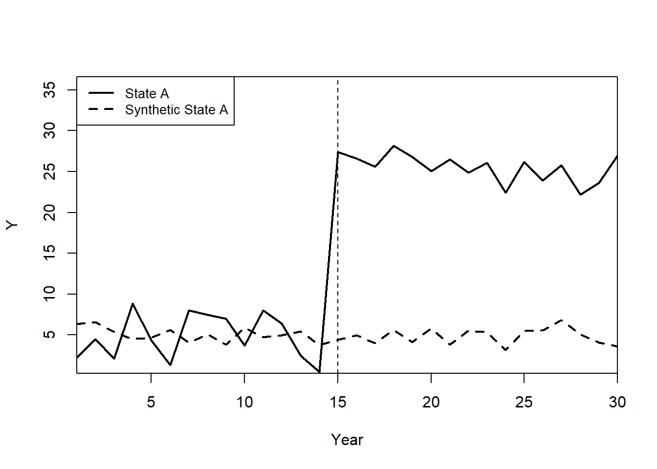
Plot: Treatment Effect (Gaps Plot)
The gaps plot shows the difference between State A and its synthetic control over time.
gaps.plot(synth.res    = synth.out,
          dataprep.res = dataprep.out,
          Ylab         = c("Gap"),
          Xlab         = c("Year"),
          Ylim         = c(-30, 30),
          Main         = ""
)

abline(v   = 15, lty = 2)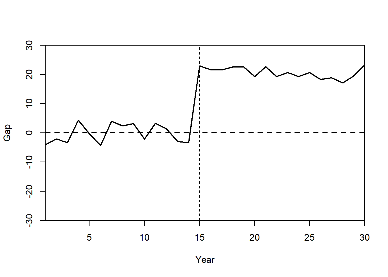
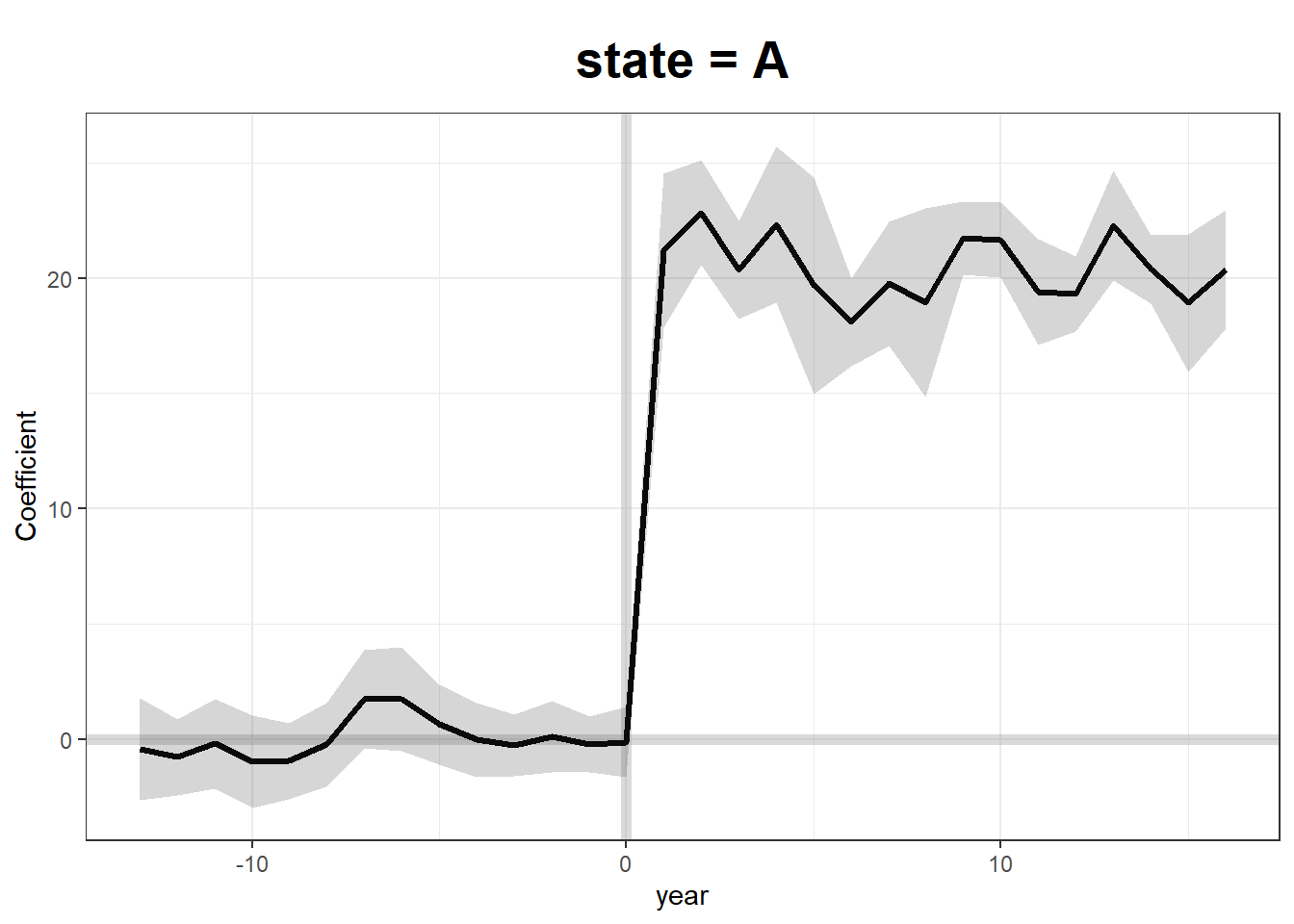
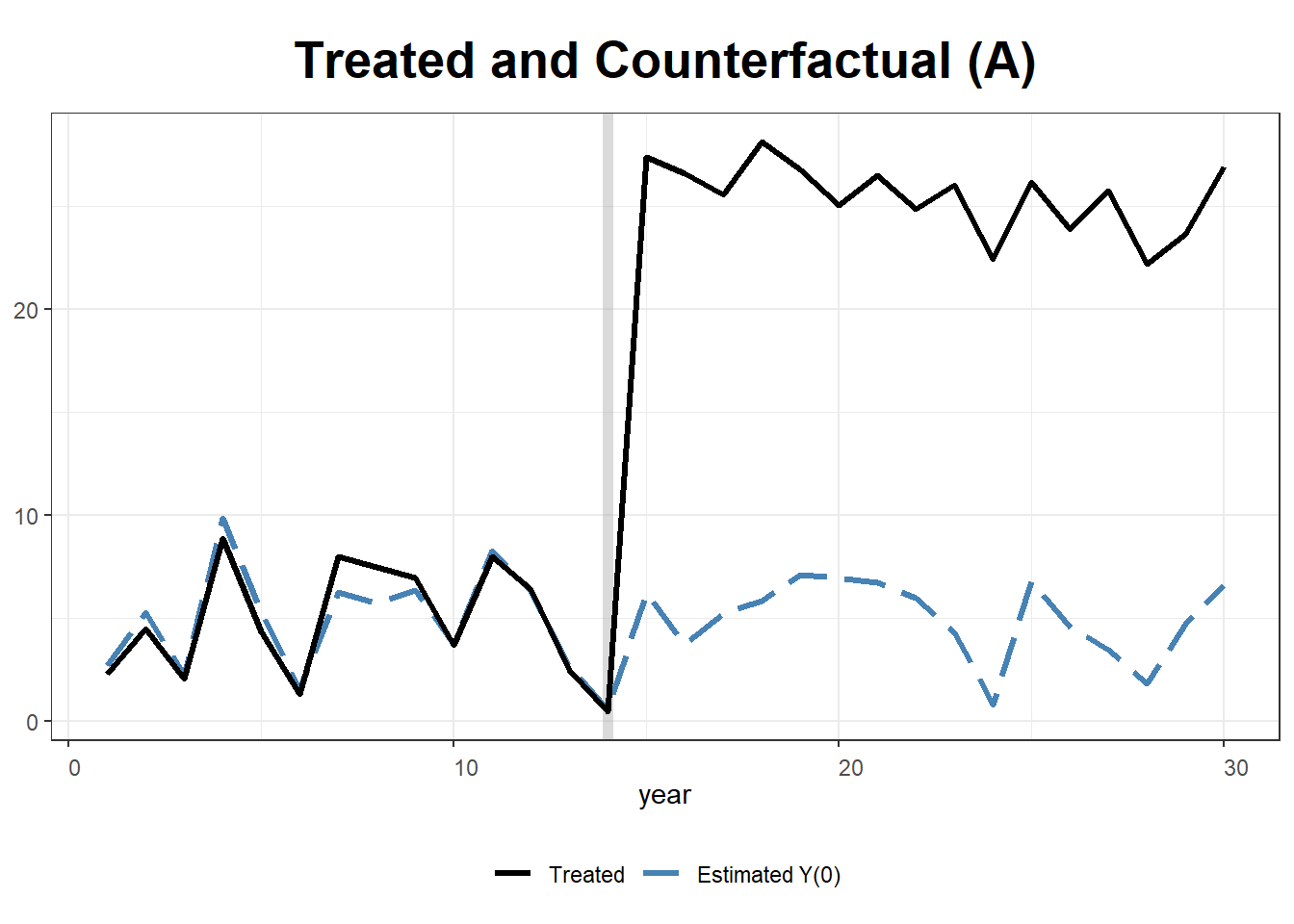
Step 2: Estimating Generalized Synthetic Control with gsynth
Unlike Synth, the gsynth package supports:
Iterative Fixed Effects (IFE) for unobserved heterogeneity.
Multiple Treated Units and Staggered Adoption.
Bootstrapped Standard Errors for inference.
Fit Generalized Synthetic Control Model
We use two-way fixed effects, cross-validation (CV = TRUE), and bootstrapped standard errors.
gsynth.out <- gsynth(
  Y ~ T + X1 + X2,
  data = df,
  index = c("state", "year"),
  force = "two-way",
  CV = TRUE,
  r = c(0, 5),
  se = TRUE,
  inference = "parametric",
  nboots = 100
)
#> Parallel computing ...
#> Cross-validating ...
#>  r = 0; sigma2 = 1.13533; IC = 0.95632; PC = 0.96713; MSPE = 1.65502
#>  r = 1; sigma2 = 0.96885; IC = 1.54420; PC = 4.30644; MSPE = 1.33375
#>  r = 2; sigma2 = 0.81855; IC = 2.08062; PC = 6.58556; MSPE = 1.27341*
#>  r = 3; sigma2 = 0.71670; IC = 2.61125; PC = 8.35187; MSPE = 1.79319
#>  r = 4; sigma2 = 0.62823; IC = 3.10156; PC = 9.59221; MSPE = 2.02301
#>  r = 5; sigma2 = 0.55497; IC = 3.55814; PC = 10.48406; MSPE = 2.79596
#>
#>  r* = 2
#>
#>
Simulating errors ...
Bootstrapping ...
#> 
32.14.2 The Basque Country Policy Change
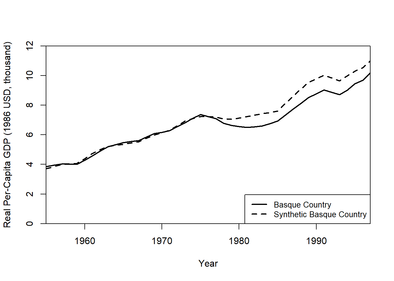
The Basque Country in Spain implemented a major policy change in 1975, impacting its GDP per capita growth. This example uses SCM to estimate the counterfactual economic performance had the policy not been implemented.
We will:
- Construct a synthetic control using economic predictors. 2
- Evaluate the policy’s impact by comparing the real and synthetic Basque GDP.
The basque dataset from Synth contains economic indicators for Spain’s regions from 1955 to 1997.
data("basque")
dim(basque)  # 774 observations, 17 variables
#> [1] 774  17
head(basque)
#>   regionno     regionname year   gdpcap sec.agriculture sec.energy sec.industry
#> 1        1 Spain (Espana) 1955 2.354542              NA         NA           NA
#> 2        1 Spain (Espana) 1956 2.480149              NA         NA           NA
#> 3        1 Spain (Espana) 1957 2.603613              NA         NA           NA
#> 4        1 Spain (Espana) 1958 2.637104              NA         NA           NA
#> 5        1 Spain (Espana) 1959 2.669880              NA         NA           NA
#> 6        1 Spain (Espana) 1960 2.869966              NA         NA           NA
#>   sec.construction sec.services.venta sec.services.nonventa school.illit
#> 1               NA                 NA                    NA           NA
#> 2               NA                 NA                    NA           NA
#> 3               NA                 NA                    NA           NA
#> 4               NA                 NA                    NA           NA
#> 5               NA                 NA                    NA           NA
#> 6               NA                 NA                    NA           NA
#>   school.prim school.med school.high school.post.high popdens invest
#> 1          NA         NA          NA               NA      NA     NA
#> 2          NA         NA          NA               NA      NA     NA
#> 3          NA         NA          NA               NA      NA     NA
#> 4          NA         NA          NA               NA      NA     NA
#> 5          NA         NA          NA               NA      NA     NA
#> 6          NA         NA          NA               NA      NA     NA
Step 1: Preparing Data for Synth
We define predictors and specify pre-treatment (1960–1969) and post-treatment (1975–1997) periods.
dataprep.out <- dataprep(
    foo = basque,
    predictors = c(
        "school.illit",
        "school.prim",
        "school.med",
        "school.high",
        "school.post.high",
        "invest"
    ),
    predictors.op = "mean",
    time.predictors.prior = 1964:1969,
    # Pre-treatment period
    special.predictors = list(
        list("gdpcap", 1960:1969, "mean"),
        list("sec.agriculture", seq(1961, 1969, 2), "mean"),
        list("sec.energy", seq(1961, 1969, 2), "mean"),
        list("sec.industry", seq(1961, 1969, 2), "mean"),
        list("sec.construction", seq(1961, 1969, 2), "mean"),
        list("sec.services.venta", seq(1961, 1969, 2), "mean"),
        list("sec.services.nonventa", seq(1961, 1969, 2), "mean"),
        list("popdens", 1969, "mean")
    ),
    dependent = "gdpcap",
    unit.variable = "regionno",
    unit.names.variable = "regionname",
    time.variable = "year",
    treatment.identifier = 17,
    # Basque region
    controls.identifier = c(2:16, 18),
    # Control regions
    time.optimize.ssr = 1960:1969,
    time.plot = 1955:1997
)
Step 2: Estimating the Synthetic Control
We now estimate the synthetic control weights using synth(). This solves for weights that best match the pre-treatment economic indicators of the Basque Country.
synth.out = synth(data.prep.obj = dataprep.out, method = "BFGS")
#>
#> X1, X0, Z1, Z0 all come directly from dataprep object.
#>
#>
#> ****************
#>  searching for synthetic control unit
#>
#>
#> ****************
#> ****************
#> ****************
#>
#> MSPE (LOSS V): 0.008864606
#>
#> solution.v:
#>  0.02773094 1.194e-07 1.60609e-05 0.0007163836 1.486e-07 0.002423908 0.0587055 0.2651997 0.02851006 0.291276 0.007994382 0.004053188 0.009398579 0.303975
#>
#> solution.w:
#>  2.53e-08 4.63e-08 6.44e-08 2.81e-08 3.37e-08 4.844e-07 4.2e-08 4.69e-08 0.8508145 9.75e-08 3.2e-08 5.54e-08 0.1491843 4.86e-08 9.89e-08 1.162e-07
Step 3: Evaluating Treatment Effects
Calculate the GDP Gap Between Real and Synthetic Basque Country
gaps = dataprep.out$Y1plot - (dataprep.out$Y0plot %*% synth.out$solution.w)
gaps[1:3,1]  # First three differences
#>       1955       1956       1957
#> 0.15023473 0.09168035 0.03716475
The synth.tab() function provides pre-treatment fit diagnostics and predictor weights.
synth.tables = synth.tab(dataprep.res = dataprep.out, synth.res = synth.out)
names(synth.tables)
#> [1] "tab.pred" "tab.v"    "tab.w"    "tab.loss"

# Predictor Balance Table
synth.tables$tab.pred[1:13,]
#>                                          Treated Synthetic Sample Mean
#> school.illit                              39.888   256.337     170.786
#> school.prim                             1031.742  2730.104    1127.186
#> school.med                                90.359   223.340      76.260
#> school.high                               25.728    63.437      24.235
#> school.post.high                          13.480    36.153      13.478
#> invest                                    24.647    21.583      21.424
#> special.gdpcap.1960.1969                   5.285     5.271       3.581
#> special.sec.agriculture.1961.1969          6.844     6.179      21.353
#> special.sec.energy.1961.1969               4.106     2.760       5.310
#> special.sec.industry.1961.1969            45.082    37.636      22.425
#> special.sec.construction.1961.1969         6.150     6.952       7.276
#> special.sec.services.venta.1961.1969      33.754    41.104      36.528
#> special.sec.services.nonventa.1961.1969    4.072     5.371       7.111
Importance of Each Control Region in the Synthetic Basque Country
synth.tables$tab.w[8:14, ]
#>    w.weights            unit.names unit.numbers
#> 9      0.000    Castilla-La Mancha            9
#> 10     0.851              Cataluna           10
#> 11     0.000  Comunidad Valenciana           11
#> 12     0.000           Extremadura           12
#> 13     0.000               Galicia           13
#> 14     0.149 Madrid (Comunidad De)           14
#> 15     0.000    Murcia (Region de)           15
Step 4: Visualizing Results
Plot Real vs. Synthetic GDP Per Capita
path.plot(
    synth.res = synth.out,
    dataprep.res = dataprep.out,
    Ylab = "Real Per-Capita GDP (1986 USD, thousand)",
    Xlab = "Year",
    Ylim = c(0, 12),
    Legend = c("Basque Country", "Synthetic Basque Country"),
    Legend.position = "bottomright"
)
Plot the Treatment Effect (GDP Gap)
gaps.plot(
    synth.res = synth.out,
    dataprep.res = dataprep.out,
    Ylab = "Gap in Real Per-Capita GDP (1986 USD, thousand)",
    Xlab = "Year",
    Ylim = c(-1.5, 1.5),
    Main = NA
)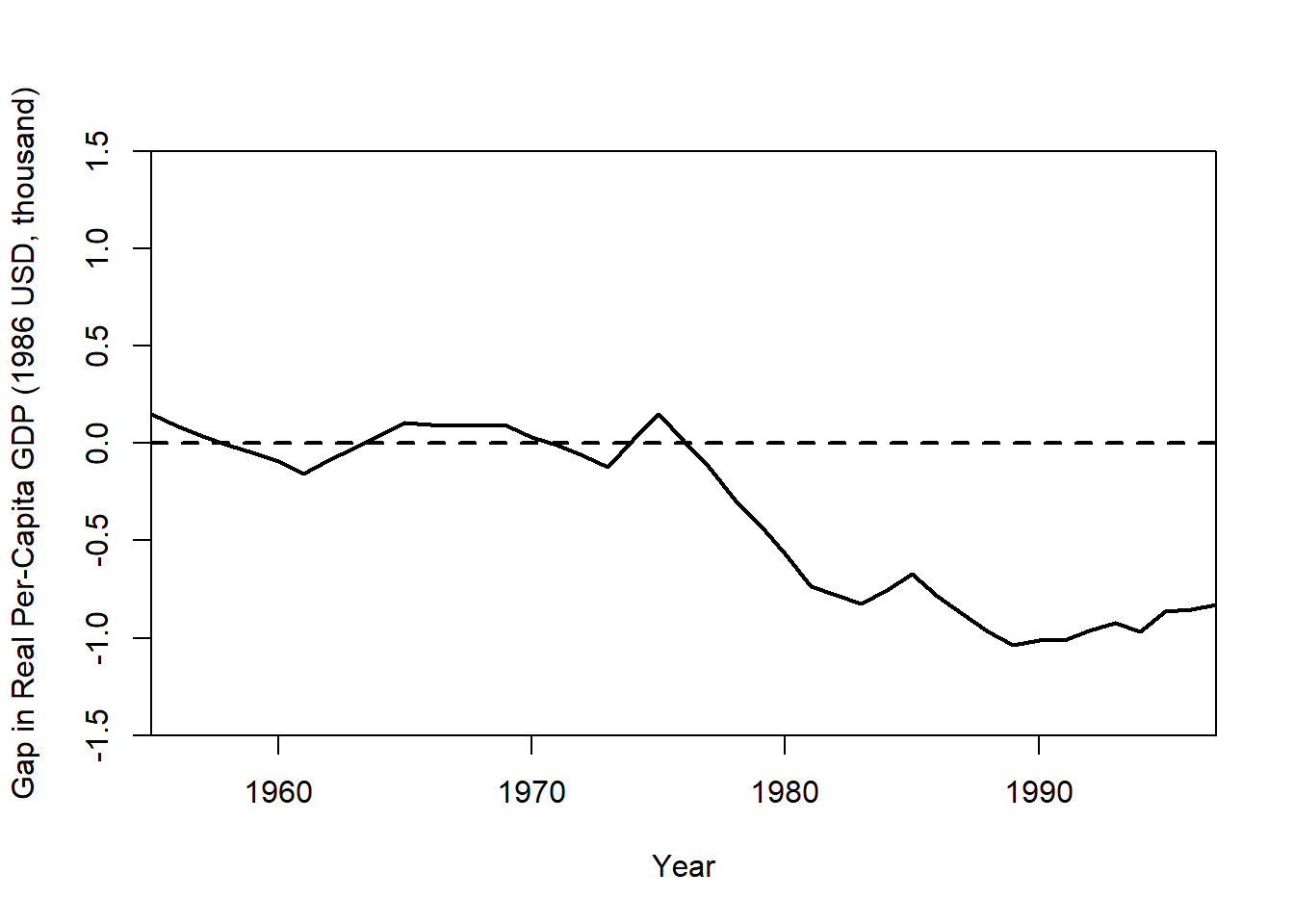
The gap plot shows the difference between actual Basque GDP and its synthetic control over time. A large post-treatment deviation suggests a policy impact.
32.14.3 Micro-Synthetic Control with microsynth
The microsynth package extends standard SCM by allowing: 1
- Matching on both predictors and time-variant outcomes. 2
- Permutation tests and jackknife resampling for placebo tests.
- Multiple follow-up periods to track long-term treatment effects.
- Omnibus test statistics for multiple outcome variables.
This example evaluates the Seattle Drug Market Initiative, a policing intervention aimed at reducing drug-related crime. The dataset seattledmi contains crime statistics across different city zones.
Step 1: Load the Required Package and Data
Step 2: Define Predictors and Outcome Variables
We specify:
Predictors (time-invariant): Population, race distribution, household data.
Outcomes (time-variant): Crime rates across different offense categories.
cov.var <- c(
    "TotalPop",
    "BLACK",
    "HISPANIC",
    "Males_1521",
    "HOUSEHOLDS",
    "FAMILYHOUS",
    "FEMALE_HOU",
    "RENTER_HOU",
    "VACANT_HOU"
)
match.out <- c("i_felony", "i_misdemea", "i_drugs", "any_crime")
Step 3: Fit the Micro-Synthetic Control Model
We first estimate treatment effects using a single follow-up period.
sea1 <- microsynth(
    seattledmi,
    idvar       = "ID",          # Unique unit identifier
    timevar     = "time",        # Time variable
    intvar      = "Intervention",# Treatment assignment
    start.pre   = 1,             # Start of pre-treatment period
    end.pre     = 12,            # End of pre-treatment period
    end.post    = 16,            # End of post-treatment period
    match.out   = match.out,     # Outcomes to match on
    match.covar = cov.var,       # Predictors to match on
    result.var  = match.out,     # Variables for treatment effect estimates
    omnibus.var = match.out,     # Variables for omnibus p-values
    test        = "lower",       # One-sided test (decrease in crime)
    n.cores     = min(parallel::detectCores() - 4, 2) # Parallel processing
)
Step 4: Summarize Results
This output provides:
Weighted unit contributions to the synthetic control.
Treatment effect estimates and confidence intervals.
p-values from permutation tests.
Step 5: Visualize the Treatment Effect
We generate a treatment effect plot comparing actual vs. synthetic trends.
Step 6: Incorporating Multiple Follow-Up Periods
We extend the analysis by adding multiple post-treatment periods (end.post = c(14, 16)) and permutation-based placebo tests (perm = 250, jack = TRUE).
sea2 <- microsynth(
    seattledmi,
    idvar       = "ID",
    timevar     = "time",
    intvar      = "Intervention",
    start.pre   = 1,
    end.pre     = 12,
    end.post    = c(14, 16), # Two follow-up periods
    match.out   = match.out,
    match.covar = cov.var,
    result.var  = match.out,
    omnibus.var = match.out,
    test        = "lower",
    perm        = 250, # Permutation placebo tests
    jack        = TRUE, # Jackknife resampling
    n.cores     = min(parallel::detectCores() - 4, 2)
)
Step 7: Placebo Testing and Robustness Checks
Permutation and jackknife tests assess whether observed treatment effects are statistically significant or due to random fluctuations.
Key robustness checks:
- Permutation Tests (
perm = 250)
1.  Reassigns treatment randomly and estimates placebo effects

2. If true effects exceed placebo effects, they are likely causal.- Jackknife Resampling (
jack = TRUE)
1.  Removes one control unit at a time and re-estimates effects.

2.  Ensures no single control dominates the synthetic match.