33.10 Long-run Event Studies

Long-horizon event studies analyze the long-term impact of corporate events on stock prices. These studies commonly assume that the distribution of abnormal returns has a mean of zero (A. Sorescu, Warren, and Ertekin 2017, 192). Moreover, A. Sorescu, Warren, and Ertekin (2017) provide evidence that samples with and without confounding events yield similar results.

However, long-run event studies face several methodological challenges:

Systematic biases over time: Estimation errors can accumulate over long periods.
Sensitivity to model specification: The choice of asset pricing models can influence results.

Long-run event studies typically use event windows of 12 to 60 months (Loughran and Ritter 1995; Brav and Gompers 1997).

There are three primary methods for measuring long-term abnormal stock returns:

Buy-and-Hold Abnormal Returns (BHAR)
Long-term Cumulative Abnormal Returns (LCARs)
Calendar-time Portfolio Abnormal Returns (CTARs), also known as Jensen’s Alpha, which better handles cross-sectional dependence and is less sensitive to asset pricing model misspecification.

Types of Events Analyzed in Long-run Studies

Unexpected changes in firm-specific variables
These events are typically not announced, may not be immediately visible to all investors, and their impact on firm value is complex. Examples include:
- The effect of customer satisfaction scores on firm value (Jacobson and Mizik 2009).
- Unexpected changes in marketing expenditures and their potential mispricing effects (M. Kim and McAlister 2011).
Events with complex consequences
Investors may take time to fully incorporate the information into stock prices. For example:
- The long-term impact of acquisitions depends on post-merger integration (A. B. Sorescu, Chandy, and Prabhu 2007).

Below is an example using the crseEventStudy package, which calculates standardized abnormal returns:

library(crseEventStudy)

# Example using demo data from the package
data(demo_returns)

SAR <- sar(event = demo_returns$EON,
           control = demo_returns$RWE,
           logret = FALSE)

mean(SAR)
#> [1] 0.006870196

33.10.1 Buy-and-Hold Abnormal Returns (BHAR)

BHAR is one of the most widely used methods in long-term event studies. It involves constructing a portfolio of benchmark stocks that closely match event firms over the same period and then comparing their returns.

Key References

(Loughran and Ritter 1995)
(Barber and Lyon 1997)
(Lyon, Barber, and Tsai 1999)

BHAR measures returns from:

Buying stocks in event firms.
Shorting stocks in similar non-event firms.

Since cross-sectional correlations can inflate t-statistics, BHAR’s rank order remains reliable even if absolute significance levels are affected (Markovitch and Golder 2008; A. B. Sorescu, Chandy, and Prabhu 2007).

To construct the benchmark portfolio, firms are matched based on:

Size
Book-to-market ratio
Momentum

Matching strategies vary across studies. Below are two common procedures:

(Barber and Lyon 1997) approach

Each July, all common stocks in the CRSP database are classified into ten deciles based on market capitalization from the previous June.
Within each size decile, firms are further grouped into five quintiles based on their book-to-market ratios as of the prior December.
The benchmark portfolio consists of non-event firms that fit these criteria.

(Wiles et al. 2010) approach

Firms in the same two-digit SIC code with market values between 50% and 150% of the focal firm are selected.
From this subset, the 10 firms with the closest book-to-market ratios form the benchmark portfolio.

Abnormal return for firm $i$ at time $t$ :

$AR_{it} = R_{it} - E(R_{it}|X_t)$

Cumulative Abnormal Return (CAR):

$CAR_{it} = \sum_{t=1}^T (R_{it} - E(R_{it}))$

Buy-and-Hold Abnormal Return (BHAR):

$BHAR_{t=1}^{T} = \prod_{t=1}^{T} (1 + R_{it}) - \prod_{t=1}^{T} (1 + E(R_{it}))$

Unlike CAR, which is arithmetic, BHAR is geometric.

In short-term studies, differences between CAR and BHAR are minimal.
In long-term studies, the discrepancy is significant. For instance, Barber and Lyon (1997) show that when annual BHAR exceeds 28%, it dramatically surpasses CAR.

To avoid favoring recent events, researchers in cross-sectional event studies typically treat all events equally when assessing their impact on the stock market over time. This approach helps in identifying abnormal changes in stock prices, particularly when analyzing a series of unplanned events.

However, long-run event studies face several biases that can distort abnormal return calculations:

Construct Benchmark Portfolios with Fixed Constituents

One recommended approach is to form benchmark portfolios that do not change their constituent firms over time (Mitchell and Stafford 2000). This helps mitigate the following biases:

New Listing Bias
Newly public companies often underperform relative to a balanced market index (Ritter 1991). Including these firms in event studies may distort long-term return expectations. This issue, termed new listing bias, was first identified by (Barber and Lyon 1997).
Rebalancing Bias
Regularly rebalancing an equal-weighted portfolio can lead to overestimated long-term returns. This is because the process systematically sells winning stocks and buys underperformers, which tends to skew buy-and-hold abnormal returns downward (Barber and Lyon 1997).
Value-Weight Bias
Value-weighted portfolios, which assign higher weights to larger market capitalization stocks, may overestimate BHARs. This approach mimics an active strategy that continuously buys winners and sells underperformers, which inflates long-run return estimates.

Buy-and-Hold Without Annual Rebalancing

Another method involves holding an initial portfolio fixed throughout the investment period. In this approach, returns are compounded, and the average is calculated across all securities:

$\Pi_{t = s}^{T} (1 + E(R_{it})) = \sum_{i=s}^{n_t} \left( w_{is} \prod_{t=1}^{T} (1 + R_{it}) \right)$

where:

$T$ = total investment period,
$R_{it}$ = return on security $i$ at time $t$ ,
$n_t$ = number of securities in the portfolio,
$w_{is}$ = initial weight of firm $i$ in the portfolio at period $s$ (either equal-weighted or value-weighted).

Key Characteristics of This Approach

No Monthly Adjustments
The portfolio remains fixed based on stocks available at time $s$ , meaning:
- No new stocks are added after period $s$ .
- No rebalancing occurs each period.
Avoids Rebalancing Bias
Since there is no forced buying or selling, distortions due to rebalancing are minimized.
Market-Weight Adjustment is Required
Since value-weighted portfolios favor larger firms, adjustments may be necessary to prevent recently listed firms from exerting excessive influence on portfolio returns.

The choice between equal-weighted and value-weighted portfolios affects results:
- Equal-weighted portfolios ensure each firm contributes equally.
- Value-weighted portfolios reflect real-world investment scenarios but may be skewed toward larger firms.
Researchers should define minimum inclusion criteria (e.g., stocks must trade for at least 12 months post-event) to filter out firms with insufficient return data.

For empirical research, Wharton Research Data Services (WRDS) provides an automated tool for computing Buy-and-Hold Abnormal Returns. This tool allows researchers to generate all types of BHAR measures based on different weighting and rebalancing approaches:

Equal-weighted vs. Value-weighted portfolios
With vs. Without annual rebalancing

The WRDS platform enables users to upload their own event data and apply these methodologies efficiently. More details can be found at WRDS Long-Run Event Study.

The WRDS tool provides several options for customizing event study settings:

Parameter	Description
MINWIN	The minimum number of months a firm must trade after the event to be included in the study.
MAXWIN	The maximum number of months considered in the event study.
MONTH	The event window length (e.g., 12, 24, or 36 months) for BHAR calculation.

If a firm’s monthly returns are missing during the selected event window, matching portfolio returns are used to fill in the gaps. This ensures that BHAR calculations remain consistent even when individual firm data is incomplete.

33.10.2 Long-term Cumulative Abnormal Returns (LCARs)

Long-term Cumulative Abnormal Returns (LCARs) measure the total abnormal return of an event firm over an extended period post-event. Unlike Buy-and-Hold Abnormal Returns, which use compounding, LCARs sum up abnormal returns over time.

This method is widely used in long-run event studies and is particularly useful for examining how an event’s impact evolves gradually rather than instantaneously.

The LCAR for firm $i$ over the post-event horizon $(1,T)$ is given by (A. B. Sorescu, Chandy, and Prabhu 2007):

$LCAR_{iT} = \sum_{t = 1}^{T} (R_{it} - R_{pt})$

where:

$R_{it}$ = Rate of return of stock $i$ in month $t$ .
$R_{pt}$ = Rate of return on the counterfactual (benchmark) portfolio in month $t$ .

LCARs aggregate monthly abnormal returns to capture the cumulative effect of an event over time.

33.10.2.1 Key Considerations in Using LCARs

Benchmark Portfolio Selection

The choice of counterfactual portfolio $R_{pt}$ is critical, as it serves as a reference point for detecting abnormal performance. Common benchmarks include:

Size and book-to-market matched portfolios
Firms are grouped based on market capitalization and book-to-market ratio to control for firm characteristics.
Industry-matched portfolios
Firms within the same industry (e.g., 2-digit SIC code) provide a relevant comparison.
Market model expectations
Expected returns are estimated using asset pricing models such as the CAPM or Fama-French 3-factor model.

Event Window Length

Long-term event studies use windows ranging from 12 to 60 months (Loughran and Ritter 1995; Brav and Gompers 1997). A longer window captures the full market reaction but increases the risk of contamination from unrelated events.

Statistical Significance Issues

Since LCARs use a simple summation of abnormal returns, they can suffer from:

Cross-sectional dependence: Abnormal returns across firms may be correlated, inflating t-statistics.
Variance drift: The standard deviation of cumulative returns grows over time, complicating inference.

To correct these biases, researchers often use:

Bootstrapping methods
Calendar-time portfolio approaches (e.g., Jensen’s Alpha)
Skewness-adjusted t-tests (Lyon, Barber, and Tsai 1999)

Feature	LCAR	BHAR
Computation	Sum of abnormal returns	Product of abnormal returns
Return Aggregation	Arithmetic	Geometric
Main Issue	Variance drift	Rebalancing bias
Best for	Identifying gradual changes in stock performance	Capturing compounding effects

In short-term studies, LCAR and BHAR tend to yield similar results, but in long-term studies, BHAR amplifies the impact of extreme returns, whereas LCAR provides a more linear view.

# Load necessary packages
library(tidyverse)
library(ggplot2)


# Simulate stock returns and benchmark portfolio returns
set.seed(123)
months <- 60  # 5-year event window
firms <- 50   # Number of event firms

# Generate random stock returns (normally distributed)
stock_returns <-
    matrix(rnorm(months * firms, mean = 0.01, sd = 0.05),
           nrow = months,
           ncol = firms)

# Generate benchmark portfolio returns
benchmark_returns <- rnorm(months, mean = 0.009, sd = 0.03)

# Compute LCAR for each firm
LCARs <-
    apply(stock_returns, 2, function(stock)
        cumsum(stock - benchmark_returns))

# Convert to data frame for visualization
LCAR_df <- as.data.frame(LCARs) %>%
    mutate(Month = 1:months) %>%
    pivot_longer(-Month, names_to = "Firm", values_to = "LCAR")

# Plot LCAR trajectories
ggplot(LCAR_df, aes(x = Month, y = LCAR, group = Firm)) +
    geom_line(alpha = 0.3) +
    theme_minimal() +
    labs(
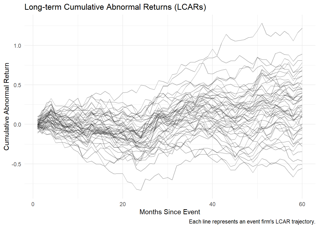
        title = "Long-term Cumulative Abnormal Returns (LCARs)",
        x = "Months Since Event",
        y = "Cumulative Abnormal Return",
        caption = "Each line represents an event firm's LCAR trajectory."
    )

33.10.3 Calendar-time Portfolio Abnormal Returns (CTARs)

The Calendar-time Portfolio Abnormal Returns (CTARs) method, also known as Jensen’s Alpha approach, is widely used in long-run event studies to address cross-sectional dependence among firms experiencing similar events. Unlike BHAR or LCAR, which focus on individual stock returns, CTARs evaluate portfolio-level abnormal returns over time.

This method follows the strict procedure outlined in Wiles et al. (2010) and has key advantages:

Controls for cross-sectional correlation by aggregating event firms into portfolios.
Reduces model misspecification biases by relying on time-series regressions instead of individual firm-level return calculations.

33.10.3.1 Constructing the Calendar-time Portfolio

Portfolio Formation
- A portfolio is constructed for every day in the calendar time (including all firms that experience an event on that day).
- Securities in each portfolio are equally weighted to avoid bias from firm size differences.
Compute the Average Abnormal Return for Each Portfolio

For a given portfolio $P$ on day $t$ :

$AAR_{Pt} = \frac{\sum_{i=1}^S AR_i}{S}$

where:

$S$ = Number of stocks in portfolio $P$ .
$AR_i$ = Abnormal return for stock $i$ in the portfolio.

Calculate the Standard Deviation of AAR over the Preceding $k$ Days

The time-series standard deviation of $AAR_{Pt}$ , denoted as $SD(AAR_{Pt})$ , is calculated using the preceding $k$ days (rolling window), assuming independence over time.
Standardize the Average Abnormal Return

$SAAR_{Pt} = \frac{AAR_{Pt}}{SD(AAR_{Pt})}$

Compute the Average Standardized Abnormal Return (ASAAR)

The standardized residuals across all portfolios are averaged across the full calendar time:

$ASAAR = \frac{1}{n} \sum_{t=1}^{255} SAAR_{Pt} \times D_t$

where:

$D_t = 1$ when at least one security is in portfolio $P_t$ , otherwise $D_t = 0$ .
$n$ is the number of days where at least one firm is in the portfolio, defined as:

$n = \sum_{t=1}^{255} D_t$

Compute the Cumulative Average Standardized Abnormal Return (CASSAR)

The cumulative impact of events over a time horizon $S_1$ to $S_2$ is given by:

$CASSAR_{S_1, S_2} = \sum_{t=S_1}^{S_2} ASAAR$

Compute the Test Statistic

If ASAAR values are independent over time, the standard deviation of the cumulative metric is:

$\sqrt{S_2 - S_1 + 1}$

Thus, the test statistic for assessing statistical significance is:

$t = \frac{CASSAR_{S_1, S_2}}{\sqrt{S_2 - S_1 + 1}}$

33.10.3.2 Limitations of the CTAR Method

While CTAR offers robust cross-sectional controls, it has notable limitations:

Cannot Examine Individual Stock Differences
- CTAR only evaluates portfolio-level differences, masking firm-level variations.
- A workaround is to construct multiple portfolios based on relevant firm characteristics (e.g., size, book-to-market, industry) and compare their intercepts.
Low Statistical Power
- CTAR has been criticized for low power (i.e., high Type II error rates) (Loughran and Ritter 2000).
- Detecting significant abnormal returns requires a large number of event firms and a sufficiently long time-series.

References

Barber, Bead M, and John D Lyon. 1997. “Firm Size, Book-to-Market Ratio, and Security Returns: A Holdout Sample of Financial Firms.” The Journal of Finance 52 (2): 875–83.

Brav, Alon, and Paul A Gompers. 1997. “Myth or Reality? The Long-Run Underperformance of Initial Public Offerings: Evidence from Venture and Nonventure Capital-Backed Companies.” The Journal of Finance 52 (5): 1791–821.

Jacobson, Robert, and Natalie Mizik. 2009. “The Financial Markets and Customer Satisfaction: Reexamining Possible Financial Market Mispricing of Customer Satisfaction.” Marketing Science 28 (5): 810–19.

Kim, MinChung, and Leigh M McAlister. 2011. “Stock Market Reaction to Unexpected Growth in Marketing Expenditure: Negative for Sales Force, Contingent on Spending Level for Advertising.” Journal of Marketing 75 (4): 68–85.

Loughran, Tim, and Jay R Ritter. 1995. “The New Issues Puzzle.” The Journal of Finance 50 (1): 23–51.

———. 2000. “Uniformly Least Powerful Tests of Market Efficiency.” Journal of Financial Economics 55 (3): 361–89.

Lyon, John D, Brad M Barber, and Chih-Ling Tsai. 1999. “Improved Methods for Tests of Long-Run Abnormal Stock Returns.” The Journal of Finance 54 (1): 165–201.

Markovitch, Dmitri G, and Peter N Golder. 2008. “Findings—Using Stock Prices to Predict Market Events: Evidence on Sales Takeoff and Long-Term Firm Survival.” Marketing Science 27 (4): 717–29.

Mitchell, Mark L, and Erik Stafford. 2000. “Managerial Decisions and Long-Term Stock Price Performance.” The Journal of Business 73 (3): 287–329.

Ritter, Jay R. 1991. “The Long-Run Performance of Initial Public Offerings.” The Journal of Finance 46 (1): 3–27.

———. 2007. “Why Some Acquisitions Do Better Than Others: Product Capital as a Driver of Long-Term Stock Returns.” Journal of Marketing Research 44 (1): 57–72.

Sorescu, Alina, Nooshin L Warren, and Larisa Ertekin. 2017. “Event Study Methodology in the Marketing Literature: An Overview.” Journal of the Academy of Marketing Science 45: 186–207.

Wiles, Michael A, Shailendra P Jain, Saurabh Mishra, and Charles Lindsey. 2010. “Stock Market Response to Regulatory Reports of Deceptive Advertising: The Moderating Effect of Omission Bias and Firm Reputation.” Marketing Science 29 (5): 828–45.