10.10 Multivariate Nonparametric Regression

Nonparametric regression in higher dimensions (\(p > 1\)) presents significant challenges compared to the univariate case. This difficulty arises primarily from the curse of dimensionality, which refers to the exponential growth of data requirements as the number of predictors increases.

10.10.1 The Curse of Dimensionality

The curse of dimensionality refers to various phenomena that occur when analyzing and organizing data in high-dimensional spaces. In the context of nonparametric regression:

Data sparsity: As the number of dimensions increases, data become sparse. Even large datasets may not adequately cover the predictor space.
Exponential sample size growth: To achieve the same level of accuracy, the required sample size grows exponentially with the number of dimensions. For example, to maintain the same density of points when moving from 1D to 2D, you need roughly the square of the sample size.

Illustration:

Consider estimating a function on the unit cube \([0,1]^p\). If we need 10 points per dimension to capture the structure:

In 1D: 10 points suffice.
In 2D: \(10^2 = 100\) points are needed.
In 10D: \(10^{10} = 10,000,000,000\) points are required.

This makes traditional nonparametric methods, like kernel smoothing, impractical in high dimensions without additional structure or assumptions.

10.10.2 Multivariate Kernel Regression

A straightforward extension of kernel regression to higher dimensions is the multivariate Nadaraya-Watson estimator:

\[ \hat{m}_h(\mathbf{x}) = \frac{\sum_{i=1}^n K_h(\mathbf{x} - \mathbf{x}_i) \, y_i}{\sum_{i=1}^n K_h(\mathbf{x} - \mathbf{x}_i)}, \]

where:

\(\mathbf{x} = (x_1, x_2, \ldots, x_p)\) is the predictor vector,
\(K_h(\cdot)\) is a multivariate kernel function, often a product of univariate kernels:

\[ K_h(\mathbf{x} - \mathbf{x}_i) = \prod_{j=1}^p K\left(\frac{x_j - x_{ij}}{h_j}\right), \]
\(h_j\) is the bandwidth for the \(j\)-th predictor.

Challenges:

The product kernel suffers from inefficiency in high dimensions because most data points are far from any given target point \(\mathbf{x}\), resulting in very small kernel weights.
Selecting an optimal multivariate bandwidth matrix is complex and computationally intensive.

10.10.3 Multivariate Splines

Extending splines to multiple dimensions involves more sophisticated techniques, as the simplicity of piecewise polynomials in 1D does not generalize easily.

10.10.3.1 Thin-Plate Splines

Thin-plate splines generalize cubic splines to higher dimensions. They minimize a smoothness penalty that depends on the derivatives of the function:

\[ \hat{m}(\mathbf{x}) = \underset{f}{\arg\min} \left\{ \sum_{i=1}^n (y_i - f(\mathbf{x}_i))^2 + \lambda \int \|\nabla^2 f(\mathbf{x})\|^2 d\mathbf{x} \right\}, \]

where \(\nabla^2 f(\mathbf{x})\) is the Hessian matrix of second derivatives, and \(\|\cdot\|^2\) represents the sum of squared elements.

Thin-plate splines are rotation-invariant and do not require explicit placement of knots, but they become computationally expensive as the number of dimensions increases.

10.10.3.2 Tensor Product Splines

For structured multivariate data, tensor product splines are commonly used. They construct a basis for each predictor and form the multivariate basis via tensor products:

\[ \hat{m}(\mathbf{x}) = \sum_{i=1}^{K_1} \sum_{j=1}^{K_2} \beta_{ij} \, B_i(x_1) \, B_j(x_2), \]

where \(B_i(x_1)\) and \(B_j(x_2)\) are spline basis functions for \(x_1\) and \(x_2\), respectively.

Tensor products allow flexible modeling of interactions between predictors but can lead to large numbers of parameters as the number of dimensions increases.

10.10.4 Additive Models (GAMs)

A powerful approach to mitigating the curse of dimensionality is to assume an additive structure for the regression function:

\[ m(\mathbf{x}) = \beta_0 + f_1(x_1) + f_2(x_2) + \cdots + f_p(x_p), \]

where each \(f_j\) is a univariate smooth function estimated nonparametrically.

10.10.4.1 Why Additive Models Help:

Dimensionality Reduction: Instead of estimating a full \(p\)-dimensional surface, we estimate \(p\) separate functions in 1D.
Interpretability: Each function \(f_j(x_j)\) represents the effect of predictor \(X_j\) on the response, holding other variables constant.

Extensions:

Interactions: Additive models can be extended to include interactions:

\[ m(\mathbf{x}) = \beta_0 + \sum_{j=1}^p f_j(x_j) + \sum_{j < k} f_{jk}(x_j, x_k), \]

where \(f_{jk}\) are bivariate smooth functions capturing interaction effects.

10.10.5 Radial Basis Functions

Radial basis functions (RBF) are another approach to multivariate nonparametric regression, particularly effective in scattered data interpolation.

A typical RBF model is:

\[ \hat{m}(\mathbf{x}) = \sum_{i=1}^n \alpha_i \, \phi(\|\mathbf{x} - \mathbf{x}_i\|), \]

where:

\(\phi(\cdot)\) is a radial basis function (e.g., Gaussian: \(\phi(r) = e^{-\gamma r^2}\)),
\(\|\mathbf{x} - \mathbf{x}_i\|\) is the Euclidean distance between \(\mathbf{x}\) and the data point \(\mathbf{x}_i\),
\(\alpha_i\) are coefficients estimated from the data.

# Load necessary libraries
library(ggplot2)
library(np)       # For multivariate kernel regression
library(mgcv)     # For thin-plate and tensor product splines
library(fields)   # For radial basis functions (RBF)
library(reshape2) # For data manipulation


# Simulate Multivariate Data
set.seed(123)
n <- 100
x1 <- runif(n, 0, 5)
x2 <- runif(n, 0, 5)
x3 <- runif(n, 0, 5)

# True nonlinear multivariate function with interaction effects
true_function <- function(x1, x2, x3) {
    sin(pi * x1) * cos(pi * x2) + exp(-((x3 - 2.5) ^ 2)) + 0.5 * x1 * x3
}

# Response with noise
y <- true_function(x1, x2, x3) + rnorm(n, sd = 0.5)

# Data frame
data_multi <- data.frame(y, x1, x2, x3)

# Visualization of marginal relationships
p1 <-
    ggplot(data_multi, aes(x1, y)) +
    geom_point(alpha = 0.5) +
    labs(title = "Effect of x1")
p2 <-
    ggplot(data_multi, aes(x2, y)) +
    geom_point(alpha = 0.5) +
    labs(title = "Effect of x2")
p3 <-
    ggplot(data_multi, aes(x3, y)) +
    geom_point(alpha = 0.5) +
    labs(title = "Effect of x3")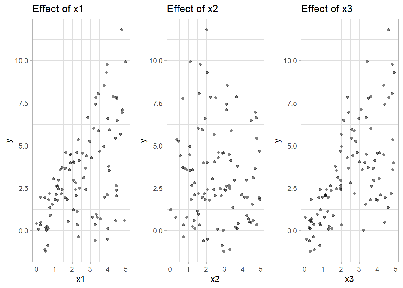

gridExtra::grid.arrange(p1, p2, p3, ncol = 3)

Three panel XY chart showing the effects of variables x1, x2, and x3 on y. Each panel displays a scatter plot with the x-axis labeled as x1, x2, and x3 respectively, and the y-axis labeled as y. The data points are scattered, showing varying relationships between each x variable and y. The charts are titled Effect of x1, Effect of x2, and Effect of x3

Figure 10.25: Scatter Plot

# Multivariate Kernel Regression using np package
bw <-
    npregbw(y ~ x1 + x2 + x3, data = data_multi)  # Bandwidth selection
#> 
Multistart 1 of 3 |
Multistart 1 of 3 |
Multistart 1 of 3 |
Multistart 1 of 3 /
Multistart 1 of 3 -
Multistart 1 of 3 |
Multistart 1 of 3 |
Multistart 1 of 3 /
Multistart 1 of 3 -
Multistart 1 of 3 \
Multistart 2 of 3 |
Multistart 2 of 3 |
Multistart 2 of 3 /
Multistart 2 of 3 -
Multistart 2 of 3 \
Multistart 2 of 3 |
Multistart 2 of 3 |
Multistart 2 of 3 |
Multistart 2 of 3 /
Multistart 3 of 3 |
Multistart 3 of 3 |
Multistart 3 of 3 /
Multistart 3 of 3 -
Multistart 3 of 3 \
Multistart 3 of 3 |
Multistart 3 of 3 |
Multistart 3 of 3 |
Multistart 3 of 3 /
                   
kernel_model <- npreg(bws = bw)

# Predict on a grid for visualization
grid_data <- expand.grid(
    x1 = seq(0, 5, length.out = 50),
    x2 = seq(0, 5, length.out = 50),
    x3 = mean(data_multi$x3)
)
pred_kernel <- predict(kernel_model, newdata = grid_data)

# Visualization
grid_data$pred <- pred_kernel

ggplot(grid_data, aes(x1, x2, fill = pred)) +
    geom_raster() +
    scale_fill_viridis_c() +
    labs(title = "Multivariate Kernel Regression (x3 fixed)",
         x = "x1",
         y = "x2") +
    theme_minimal()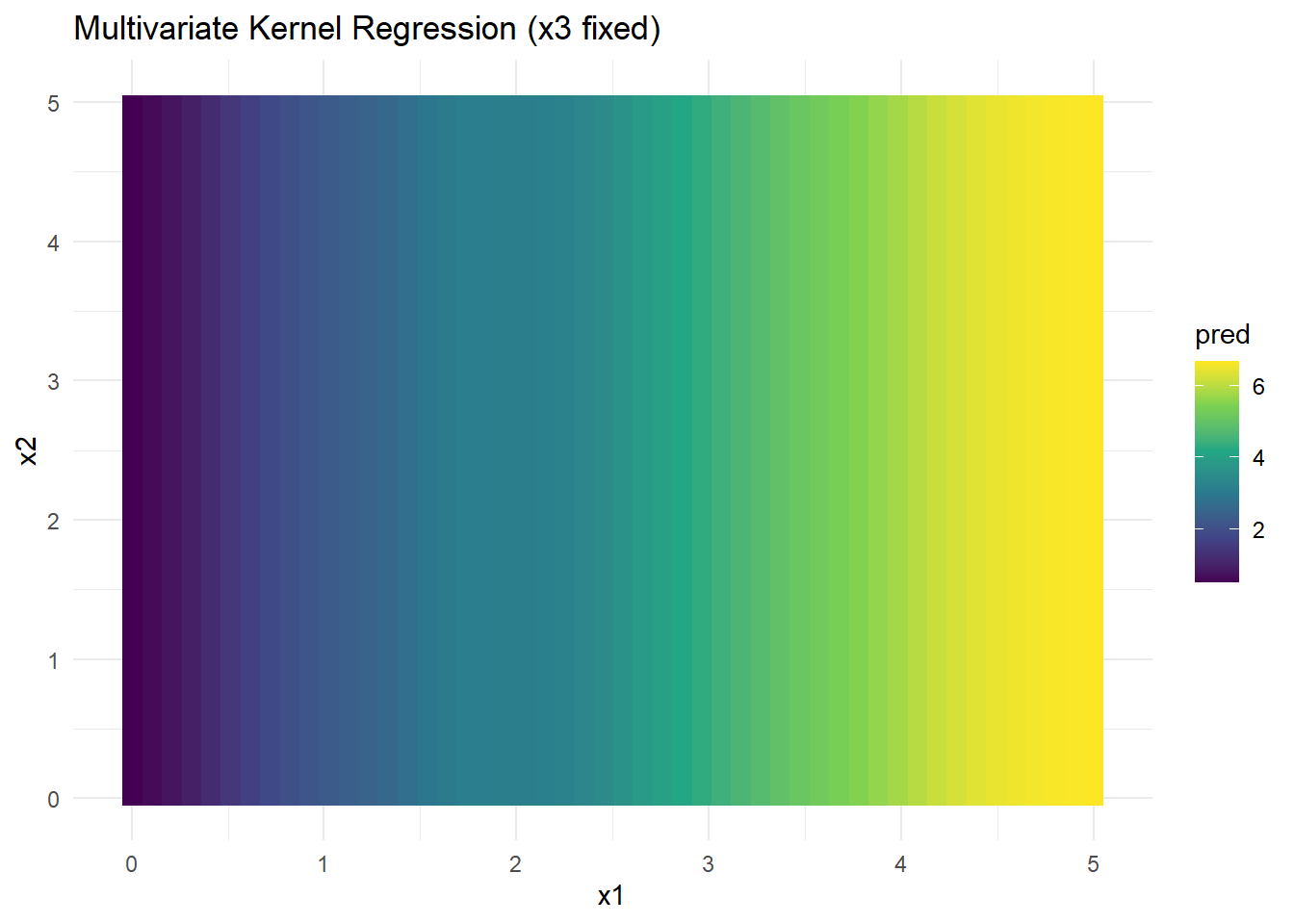

Heatmap illustrating multivariate kernel regression with x3 fixed. The x-axis represents x1, and the y-axis represents x2, both ranging from 0 to 5. The color gradient transitions from purple to yellow, indicating prediction values from 2 to 6, as shown in the legend on the right.

Figure 2.13: Multivariate Kernel Regression (x3 fixed)

Kernel regression captures nonlinear interactions but suffers from data sparsity in high dimensions (curse of dimensionality).
Bandwidth selection is critical for performance.

# Fit Thin-Plate Spline
tps_model <- gam(y ~ s(x1, x2, x3, bs = "tp", k = 5), data = data_multi)

# Predictions
grid_data$pred_tps <- predict(tps_model, newdata = grid_data)

# Visualization
ggplot(grid_data, aes(x1, x2, fill = pred_tps)) +
    geom_raster() +
    scale_fill_viridis_c() +
    labs(title = "Thin-Plate Spline (x3 fixed)",
         x = "x1", y = "x2") +
    theme_minimal()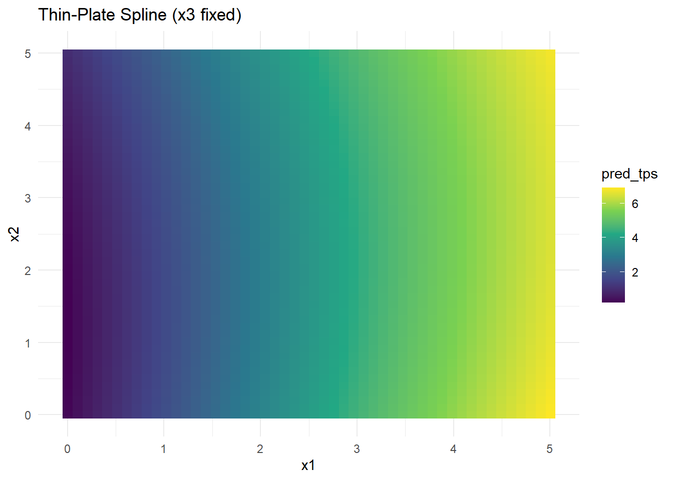

Heatmap titled Thin-Plate Spline x3 fixed displaying a gradient of colors from dark purple to yellow. The x-axis is labeled x1 and ranges from 0 to 5. The y-axis is labeled x2 and ranges from 0 to 5. A color scale on the right labeled pred_tps indicates values from 2 to 6. The heatmap visualizes data variation across the x1 and x2 axes

Figure 10.26: Thin-Plate Spline (x3 fixed)

Thin-plate splines handle smooth surfaces well and are rotation-invariant.
Computational cost increases with higher dimensions due to matrix operations.

# Fit Tensor Product Spline
tensor_model <- gam(y ~ te(x1, x2, x3), data = data_multi)

# Predictions
grid_data$pred_tensor <- predict(tensor_model, newdata = grid_data)

# Visualization
ggplot(grid_data, aes(x1, x2, fill = pred_tensor)) +
    geom_raster() +
    scale_fill_viridis_c() +
    labs(title = "Tensor Product Spline (x3 fixed)",
         x = "x1", y = "x2") +
    theme_minimal()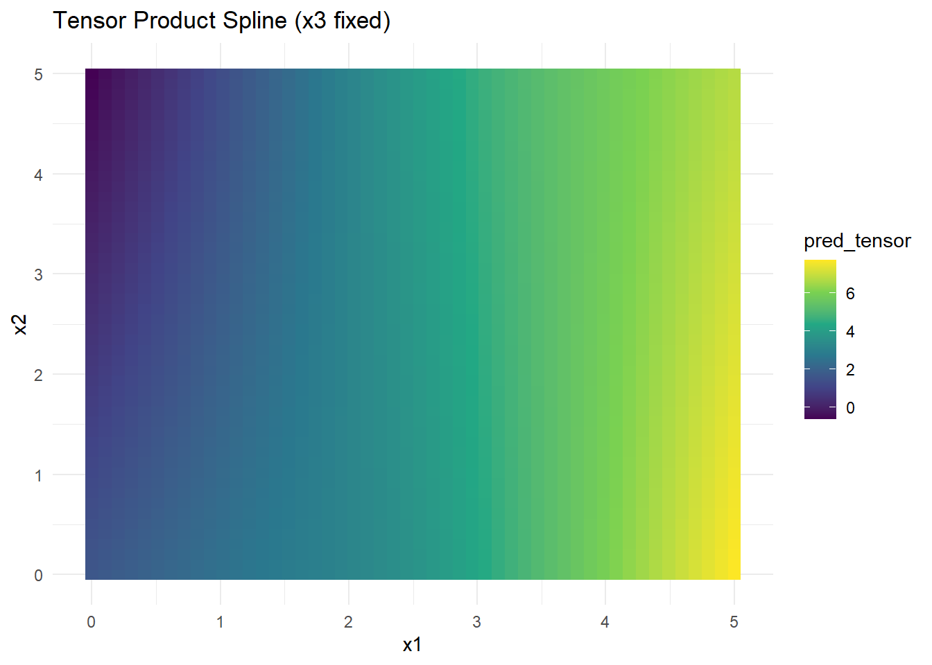

Heatmap titled Tensor Product Spline x3 fixed displaying a gradient of colors from purple to yellow. The x-axis is labeled x1 and ranges from 0 to 5. The y-axis is labeled x2 and also ranges from 0 to 5. A color scale on the right labeled pred_tensor indicates values from 0 to 6, with darker colors representing lower values and lighter colors representing higher values

Figure 10.27: Tensor Product Spline (x3 fixed)

Tensor product splines model interactions explicitly between variables.
Suitable when data have structured dependencies but can lead to many parameters in higher dimensions.

# Additive Model (GAM)
gam_model <- gam(y ~ s(x1) + s(x2) + s(x3), data = data_multi)

# Predictions
grid_data$pred_gam <- predict(gam_model, newdata = grid_data)

# Visualization
ggplot(grid_data, aes(x1, x2, fill = pred_gam)) +
    geom_raster() +
    scale_fill_viridis_c() +
    labs(title = "Additive Model (GAM, x3 fixed)", 
         x = "x1", y = "x2") +
    theme_minimal()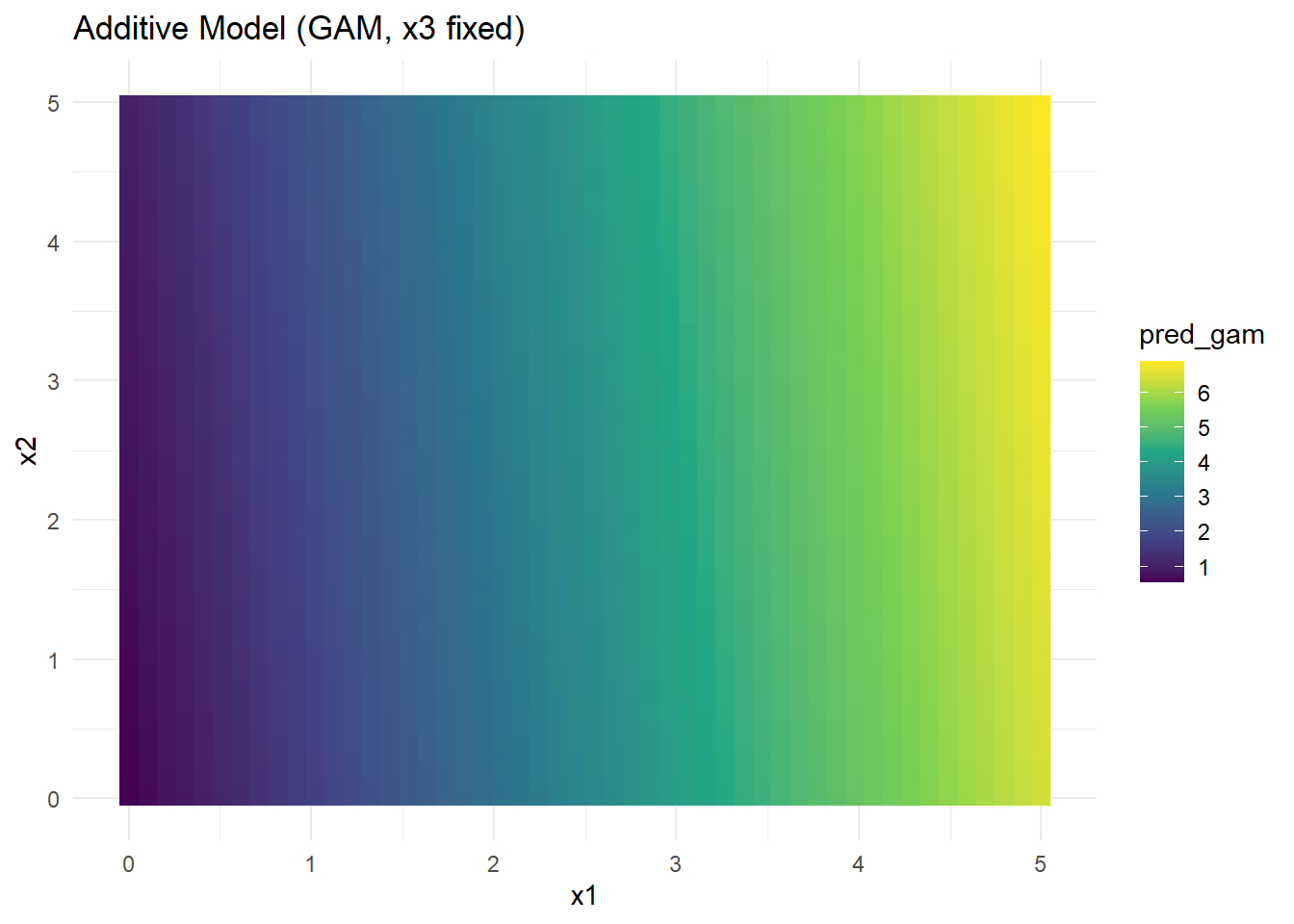

Heatmap illustrating an additive model GAM with x3 fixed. The x-axis represents variable x1 and the y-axis represents variable x2, both ranging from 0 to 5. The color gradient transitions from purple to yellow, indicating values of the predicted GAM labeled as pred_gam, with a scale from 1 to 6

Figure 10.28: Additive Model (GAM, x3 fixed)

Why GAMs Help:

Dimensionality reduction: Instead of estimating a full multivariate function, GAM estimates separate 1D functions for each predictor.
Interpretability: Easy to understand individual effects.
Limitations: Cannot capture complex interactions unless explicitly added.

# Radial Basis Function Model
rbf_model <- Tps(cbind(x1, x2, x3), y)  # Thin-plate spline RBF
#> Warning: 
#> Grid searches over lambda (nugget and sill variances) with  minima at the endpoints: 
#>   (GCV) Generalized Cross-Validation 
#>    minimum at  right endpoint  lambda  =  0.0002622876 (eff. df= 95.00001 )

# Predictions
grid_data$pred_rbf <-
    predict(rbf_model, cbind(grid_data$x1, grid_data$x2, grid_data$x3))

# Visualization
ggplot(grid_data, aes(x1, x2, fill = pred_rbf)) +
    geom_raster() +
    scale_fill_viridis_c() +
    labs(title = "Radial Basis Function Regression (x3 fixed)", 
         x = "x1", y = "x2") +
    theme_minimal()

Heatmap illustrating Radial Basis Function Regression with x3 fixed. The x-axis represents x1, and the y-axis represents x2. The color gradient ranges from purple to yellow, indicating varying levels of the predicted RBF values, labeled as pred_rbf, with a scale from 2 to 6.

Figure 2.14: Radial Basis Function Regression (x3 fixed)

RBFs capture complex, smooth surfaces and interactions based on distance.
Perform well for scattered data but can be computationally expensive for large datasets.

# Compute Mean Squared Error for each model
mse_kernel <- mean((predict(kernel_model) - data_multi$y) ^ 2)
mse_tps <- mean((predict(tps_model) - data_multi$y) ^ 2)
mse_tensor <- mean((predict(tensor_model) - data_multi$y) ^ 2)
mse_gam <- mean((predict(gam_model) - data_multi$y) ^ 2)
mse_rbf <-
    mean((predict(rbf_model, cbind(x1, x2, x3)) - data_multi$y) ^ 2)

# Display MSE comparison
data.frame(
    Model = c(
        "Kernel Regression",
        "Thin-Plate Spline",
        "Tensor Product Spline",
        "Additive Model (GAM)",
        "Radial Basis Functions"
    ),
    MSE = c(mse_kernel, mse_tps, mse_tensor, mse_gam, mse_rbf)
)
#>                    Model         MSE
#> 1      Kernel Regression 0.253019836
#> 2      Thin-Plate Spline 0.449096723
#> 3  Tensor Product Spline 0.304680406
#> 4   Additive Model (GAM) 1.595616092
#> 5 Radial Basis Functions 0.001361915