10.4 Local Polynomial Regression
While the Nadaraya-Watson estimator is effectively a local constant estimator (it approximates \(m(x)\) by a constant in a small neighborhood of \(x\)), local polynomial regression extends this idea by fitting a local polynomial around each point \(x\). The advantage of local polynomials is that they can better handle boundary bias and can capture local curvature more effectively.
10.4.1 Local Polynomial Fitting
A local polynomial regression of degree \(p\) at point \(x\) estimates a polynomial function:
\[ m_x(t) = \beta_0 + \beta_1 (t - x) + \beta_2 (t - x)^2 + \cdots + \beta_p (t - x)^p \]
that best fits the data \(\{(x_i, y_i)\}\) within a neighborhood of \(x\), weighted by a kernel. Specifically, we solve:
\[ (\hat{\beta}_0, \hat{\beta}_1, \ldots, \hat{\beta}_p) = \underset{\beta_0, \ldots, \beta_p}{\arg\min} \sum_{i=1}^n \left[y_i - \left\{\beta_0 + \beta_1 (x_i - x) + \cdots + \beta_p (x_i - x)^p\right\}\right]^2 K\!\left(\frac{x_i - x}{h}\right). \]
We then estimate:
\[ \hat{m}(x) = \hat{\beta}_0, \]
because \(\beta_0\) is the constant term of the local polynomial expansion around \(x\), which represents the estimated value at that point.
Why center the polynomial at \(x\) rather than 0?
Centering at \(x\) ensures that the fitted polynomial provides the best approximation around \(x\). This is conceptually similar to a Taylor expansion, where local approximations are most accurate near the point of expansion.
10.4.2 Mathematical Form of the Solution
Let \(\mathbf{X}_x\) be the design matrix for the local polynomial expansion at point \(x\). For a polynomial of degree \(p\), each row \(i\) of \(\mathbf{X}_x\) is:
\[ \left(1, x_i - x, (x_i - x)^2, \ldots, (x_i - x)^p \right). \]
Define \(\mathbf{W}_x\) as the diagonal matrix with entries:
\[ (\mathbf{W}_x)_{ii} = K\!\left(\frac{x_i - x}{h}\right), \]
representing the kernel weights. The parameter vector \(\boldsymbol{\beta} = (\beta_0, \beta_1, \ldots, \beta_p)^T\) is estimated via weighted least squares:
\[ \hat{\boldsymbol{\beta}}(x) = \left(\mathbf{X}_x^T \mathbf{W}_x \mathbf{X}_x\right)^{-1} \mathbf{X}_x^T \mathbf{W}_x \mathbf{y}, \]
where \(\mathbf{y} = (y_1, y_2, \ldots, y_n)^T\). The local polynomial estimator of \(m(x)\) is given by:
\[ \hat{m}(x) = \hat{\beta}_0(x). \]
Alternatively, we can express this concisely using a selection vector:
\[ \hat{m}(x) = \mathbf{e}_1^T \left(\mathbf{X}_x^T \mathbf{W}_x \mathbf{X}_x\right)^{-1} \mathbf{X}_x^T \mathbf{W}_x \mathbf{y}, \]
where \(\mathbf{e}_1 = (1, 0, \ldots, 0)^T\) picks out the intercept term.
10.4.3 Bias, Variance, and Asymptotics
Local polynomial estimators have well-characterized bias and variance properties, which depend on the polynomial degree \(p\), the bandwidth \(h\), and the smoothness of the true regression function \(m(x)\).
10.4.3.1 Bias
The leading bias term is proportional to \(h^{p+1}\) and involves the \((p+1)\)-th derivative of \(m(x)\):
\[ \operatorname{Bias}\left[\hat{m}(x)\right] \approx \frac{h^{p+1}}{(p+1)!} m^{(p+1)}(x) \cdot B(K, p), \]
where \(B(K, p)\) is a constant depending on the kernel and the polynomial degree.
For local linear regression (\(p=1\)), the bias is of order \(O(h^2)\), while for local quadratic regression (\(p=2\)), it’s of order \(O(h^3)\).
10.4.3.2 Variance
The variance is approximately:
\[ \operatorname{Var}\left[\hat{m}(x)\right] \approx \frac{\sigma^2}{n h} \cdot V(K, p), \]
where \(\sigma^2\) is the error variance, and \(V(K, p)\) is another kernel-dependent constant.
The variance decreases with larger \(n\) and larger \(h\), but increasing \(h\) also increases bias, illustrating the classic bias-variance trade-off.
10.4.3.3 Boundary Issues
One of the key advantages of local polynomial regression—especially local linear regression—is its ability to reduce boundary bias, which is a major issue for the Nadaraya-Watson estimator. This is because the linear term allows the fit to adjust for slope changes near the boundaries, where the kernel becomes asymmetric due to fewer data points on one side.
10.4.4 Special Case: Local Linear Regression
Local linear regression (often called a local polynomial fit of degree 1) is particularly popular because:
- It mitigates boundary bias effectively, making it superior to Nadaraya-Watson near the edges of the data.
- It remains computationally simple yet provides better performance than local-constant (degree 0) models.
- It is robust to heteroscedasticity, as it adapts to varying data densities.
The resulting estimator for \(\hat{m}(x)\) simplifies to:
\[ \hat{m}(x) = \frac{S_{2}(x)S_{0y}(x) - S_{1}(x)S_{1y}(x)} {S_{0}(x)S_{2}(x) - S_{1}^2(x)}, \]
where
\[ S_k(x) = \sum_{i=1}^n (x_i - x)^k K\left(\tfrac{x_i - x}{h}\right) \]
\[ S_{k y}(x) = \sum_{i=1}^n (x_i - x)^k y_i K\!\left(\tfrac{x_i - x}{h}\right). \]
To see why the local linear fit helps reduce bias, consider approximating \(m\) around the point \(x\) via a first-order Taylor expansion:
\[ m(t) \approx m(x) + m'(x)(t - x). \]
When we perform local linear regression, we solve the weighted least squares problem
\[ \min_{\beta_0, \beta_1} \sum_{i=1}^n \left[y_i - \left\{\beta_0 + \beta_1 (x_i - x)\right\}\right]^2 K\left(\tfrac{x_i - x}{h}\right). \]
If we assume \(y_i = m(x_i) + \varepsilon_i\), then expanding \(m(x_i)\) in a Taylor series around \(x\) gives:
\[ m(x_i) = m(x) + m'(x)(x_i - x) + \tfrac{1}{2}m''(x)(x_i - x)^2 + \cdots. \]
For \(x_i\) close to \(x\), the higher-order terms may be small, but they contribute to the bias if we truncate at the linear term.
Let us denote:
\[ \begin{aligned} S_0(x) &= \sum_{i=1}^n K\left(\frac{x_i - x}{h}\right), \\ S_1(x) &= \sum_{i=1}^n (x_i - x) K\left(\frac{x_i - x}{h}\right), \\ S_2(x) &= \sum_{i=1}^n (x_i - x)^2 K\left(\frac{x_i - x}{h}\right).\end{aligned} \]
Similarly, define \[ \sum_{i=1}^n y_iK\!\left(\tfrac{x_i - x}{h}\right) \quad\text{and}\quad \sum_{i=1}^n (x_i - x)y_iK\!\left(\tfrac{x_i - x}{h}\right) \] for the right-hand sides. The estimated coefficients \(\hat{\beta}_0\) and \(\hat{\beta}_1\) are found by solving:
\[ \begin{pmatrix} S_0(x) & S_1(x)\\ S_1(x) & S_2(x) \end{pmatrix} \begin{pmatrix} \hat{\beta}_0 \\ \hat{\beta}_1 \end{pmatrix} = \begin{pmatrix} \sum_{i=1}^n y_i K\!\left(\tfrac{x_i - x}{h}\right)\\ \sum_{i=1}^n (x_i - x)y_i K\!\left(\tfrac{x_i - x}{h}\right) \end{pmatrix}. \]
Once \(\hat{\beta}_0\) and \(\hat{\beta}_1\) are found, we identify \(\hat{m}(x) = \hat{\beta}_0\).
By substituting the Taylor expansion \(y_i = m(x_i) + \varepsilon_i\) and taking expectations, one can derive how the “extra” \(\tfrac12m''(x)(x_i - x)^2\) terms feed into the local fit’s bias.
From these expansions and associated algebra, one finds:
- Bias: The leading bias term for local linear regression is typically on the order of \(h^2\), often written as \(\tfrac12m''(x)\mu_2(K)h^2\) for some constant \(\mu_2(K)\) depending on the kernel’s second moment.
- Variance: The leading variance term at a single point \(x\) is on the order of \(\tfrac{1}{nh}\).
Balancing these two orders of magnitude—i.e., setting \(h^2 \sim \tfrac{1}{nh}\)—gives \(h \sim n^{-1/3}\). Consequently, the mean squared error at \(x\) then behaves like
\[ \left(\hat{m}(x) - m(x)\right)^2 = O_p\!\left(n^{-2/3}\right). \]
While local constant (Nadaraya–Watson) and local linear estimators often have the same interior rate, the local linear approach can eliminate leading-order bias near the boundaries, making it preferable in many practical settings.
10.4.5 Bandwidth Selection
Just like in kernel regression, the bandwidth \(h\) controls the smoothness of the local polynomial estimator.
- Small \(h\): Captures fine local details but increases variance (potential overfitting).
- Large \(h\): Smooths out noise but may miss important local structure (potential underfitting).
10.4.5.1 Cross-Validation for Local Polynomial Regression
Bandwidth selection via cross-validation is also common here. The leave-one-out CV criterion is:
\[ \mathrm{CV}(h) = \frac{1}{n} \sum_{i=1}^n \left(y_i - \hat{m}_{-i,h}(x_i)\right)^2, \]
where \(\hat{m}_{-i,h}(x_i)\) is the estimate at \(x_i\) obtained by leaving out the \(i\)-th observation.
Alternatively, for local linear regression, computational shortcuts (like generalized cross-validation) can significantly speed up bandwidth selection.
| Aspect | Nadaraya-Watson (Local Constant) | Local Polynomial Regression |
|---|---|---|
| Bias at boundaries | High | Reduced (especially for \(p=1\)) |
| Flexibility | Limited (constant fit) | Captures local trends (linear/quadratic) |
| Complexity | Simpler | Slightly more complex (matrix operations) |
| Robustness to heteroscedasticity | Lower | Higher (adapts better to varying densities) |
10.4.6 Asymptotic Properties Summary
- Consistency: \(\hat{m}(x) \overset{p}{\longrightarrow} m(x)\) as \(n \to \infty\), under mild conditions.
- Rate of Convergence: For local linear regression, the MSE converges at rate \(O(n^{-4/5})\), similar to kernel regression, but with better performance at boundaries.
- Optimal Bandwidth: Balances bias (\(O(h^{p+1})\)) and variance (\(O(1/(nh))\)), with cross-validation as a practical selection method.
# Load necessary libraries
library(ggplot2)
library(gridExtra)

# 1. Simulate Data
set.seed(123)

# Generate predictor x and response y
n <- 100
x <- sort(runif(n, 0, 10))  # Sorted for local regression
true_function <-
    function(x)
        sin(x) + 0.5 * cos(2 * x)  # True regression function
y <-
    true_function(x) + rnorm(n, sd = 0.3) # Add Gaussian noise
# Visualization of the data
ggplot(data.frame(x, y), aes(x, y)) +
geom_point(color = "darkblue") +
geom_line(aes(y = true_function(x)),
color = "red",
linetype = "dashed") +
labs(title = "Simulated Data with True Regression Function",
x = "x", y = "y") +
theme_minimal()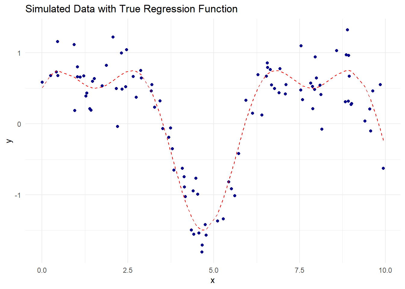
Figure 10.7: Simulated Data with True Regression Function
# Gaussian Kernel Function
gaussian_kernel <- function(u) {
    (1 / sqrt(2 * pi)) * exp(-0.5 * u ^ 2)
}

# Local Polynomial Regression Function
local_polynomial_regression <-
    function(x_eval,
             x,
             y,
             h,
             p = 1,
             kernel = gaussian_kernel) {
        sapply(x_eval, function(x0) {
            # Design matrix for polynomial of degree p
            X <- sapply(0:p, function(k)
                (x - x0) ^ k)

            # Kernel weights
            W <- diag(kernel((x - x0) / h))

            # Weighted least squares estimation
            beta_hat <- solve(t(X) %*% W %*% X, t(X) %*% W %*% y)

            # Estimated value at x0 (intercept term)
            beta_hat[1]
        })
    }

# Evaluation grid
x_grid <- seq(0, 10, length.out = 200)

# Apply Local Linear Regression (p = 1)
h_linear <- 0.8
llr_estimate <-
    local_polynomial_regression(x_grid, x, y, h = h_linear, p = 1)

# Apply Local Quadratic Regression (p = 2)
h_quadratic <- 0.8
lqr_estimate <-
    local_polynomial_regression(x_grid, x, y, h = h_quadratic, p = 2)
# Plot Local Linear Regression
p1 <- ggplot() +
geom_point(aes(x, y), color = "darkblue", alpha = 0.6) +
geom_line(aes(x_grid, llr_estimate),
color = "green",
size = 1.2) +
geom_line(aes(x_grid, true_function(x_grid)),
color = "red",
linetype = "dashed") +
labs(
title = "Local Linear Regression (p = 1)",
subtitle = paste("Bandwidth (h) =", h_linear),
x = "x",
y = "Estimated m(x)"
) +
theme_minimal()
# Plot Local Quadratic Regression
p2 <- ggplot() +
geom_point(aes(x, y), color = "darkblue", alpha = 0.6) +
geom_line(aes(x_grid, lqr_estimate),
color = "orange",
size = 1.2) +
geom_line(aes(x_grid, true_function(x_grid)),
color = "red",
linetype = "dashed") +
labs(
title = "Local Quadratic Regression (p = 2)",
subtitle = paste("Bandwidth (h) =", h_quadratic),
x = "x",
y = "Estimated m(x)"
) +
theme_minimal()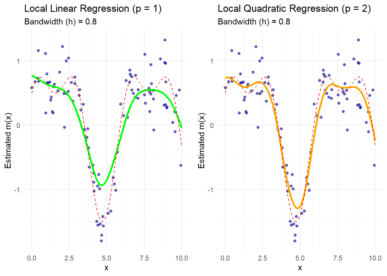
Figure 10.8: Comparison of Local Regression
The green curve represents the local linear regression estimate.
The orange curve represents the local quadratic regression estimate.
The dashed red line is the true regression function.
Boundary effects are better handled by local polynomial methods, especially with quadratic fits that capture curvature more effectively.
# Leave-One-Out Cross-Validation for Bandwidth Selection
cv_bandwidth_lp <- function(h, x, y, p = 1, kernel = gaussian_kernel) {
  n <- length(y)
  cv_error <- 0

  for (i in 1:n) {
    # Leave-one-out data
    x_train <- x[-i]
    y_train <- y[-i]

    # Predict the left-out point
    y_pred <-
      local_polynomial_regression(x[i],
                                  x_train,
                                  y_train,
                                  h = h,
                                  p = p,
                                  kernel = kernel)

    # Accumulate squared error
    cv_error <- cv_error + (y[i] - y_pred)^2
  }

  return(cv_error / n)
}

# Bandwidth grid for optimization
bandwidths <- seq(0.1, 2, by = 0.1)

# Cross-validation errors for local linear regression
cv_errors_linear <- sapply(bandwidths, cv_bandwidth_lp, x = x, y = y, p = 1)

# Cross-validation errors for local quadratic regression
cv_errors_quadratic <- sapply(bandwidths, cv_bandwidth_lp, x = x, y = y, p = 2)

# Optimal bandwidths
optimal_h_linear <- bandwidths[which.min(cv_errors_linear)]
optimal_h_quadratic <- bandwidths[which.min(cv_errors_quadratic)]

# Display optimal bandwidths
optimal_h_linear
#> [1] 0.4
optimal_h_quadratic
#> [1] 0.7
# CV Error Plot for Linear and Quadratic Fits
cv_data <- data.frame(
Bandwidth = rep(bandwidths, 2),
CV_Error = c(cv_errors_linear, cv_errors_quadratic),
Degree = rep(c("Linear (p=1)", "Quadratic (p=2)"),
each = length(bandwidths))
)ggplot(cv_data, aes(x = Bandwidth, y = CV_Error, color = Degree)) +
geom_line(size = 1) +
geom_point(
data = subset(
cv_data,
Bandwidth %in% c(optimal_h_linear, optimal_h_quadratic)
),
aes(x = Bandwidth, y = CV_Error),
color = "red",
size = 3
) +
labs(
title = "Cross-Validation for Bandwidth Selection",
subtitle = "Red points indicate optimal bandwidths",
x = "Bandwidth (h)",
y = "CV Error"
) +
theme_minimal() +
scale_color_manual(values = c("green", "orange"))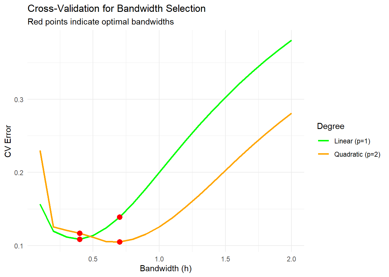
Figure 10.9: Cross-Validation for Bandwidth Selection
The optimal bandwidth minimizes the cross-validation error.
The red points mark the bandwidths that yield the lowest errors for linear and quadratic fits.
Smaller bandwidths can overfit, while larger bandwidths may oversmooth.
# Apply Local Polynomial Regression with Optimal Bandwidths
final_llr_estimate <-
    local_polynomial_regression(x_grid, x, y, h = optimal_h_linear, p = 1)
final_lqr_estimate <-
    local_polynomial_regression(x_grid, x, y, h = optimal_h_quadratic, p = 2)
# Plot final fits
ggplot() +
geom_point(aes(x, y), color = "gray60", alpha = 0.5) +
geom_line(
aes(x_grid, final_llr_estimate, color = "Linear Estimate"),
size = 1.2,
linetype = "solid"
) +
geom_line(
aes(x_grid, final_lqr_estimate, color = "Quadratic Estimate"),
size = 1.2,
linetype = "solid"
) +
geom_line(
aes(x_grid, true_function(x_grid), color = "True Function"),
linetype = "dashed"
) +
labs(
x = "x",
y = "Estimated m(x)",
color = "Legend" # Add a legend title
) +
scale_color_manual(
values = c(
"Linear Estimate" = "green",
"Quadratic Estimate" = "orange",
"True Function" = "red"
)
) +
theme_minimal()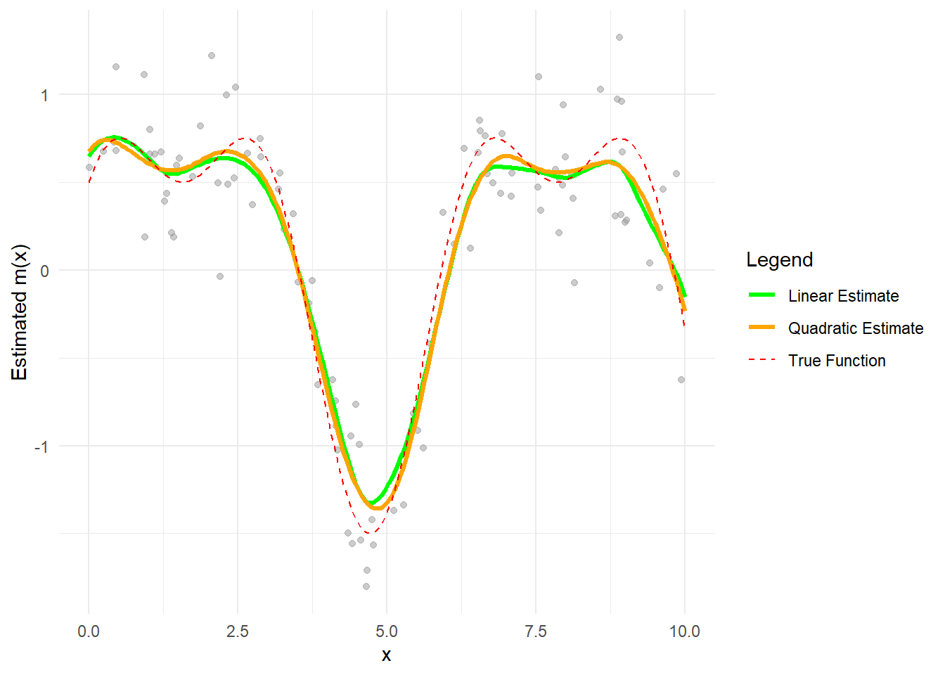
Figure 10.10: Line Comparison between Linear and Quadratic Estimates