12.1 Continuous Variables
Transforming continuous variables can be useful for various reasons, including:
- Changing the scale of variables to make them more interpretable or comparable.
- Reducing skewness to approximate a normal distribution, which can improve statistical inference.
- Stabilizing variance in cases of heteroskedasticity.
- Enhancing interpretability in business applications (e.g., logarithmic transformations for financial data).
12.1.1 Standardization (Z-score Normalization)
A common transformation to center and scale data:
\[ x_i' = \frac{x_i - \bar{x}}{s} \]
where:
- \(x_i\) is the original value,
- \(\bar{x}\) is the sample mean,
- \(s\) is the sample standard deviation.
When to Use:
When variables have different units of measurement and need to be on a common scale.
When a few large numbers dominate the dataset.
12.1.2 Min-Max Scaling (Normalization)
Rescales data to a fixed range, typically \([0,1]\):
\[ x_i' = \frac{x_i - x_{\min}}{x_{\max} - x_{\min}} \]
When to Use:
When working with fixed-interval data (e.g., percentages, proportions).
When preserving relative relationships between values is important.
Caution: This method is sensitive to outliers, as extreme values determine the range.
12.1.3 Square Root and Cube Root Transformations
Useful for handling positive skewness and heteroskedasticity:
- Square root: Reduces moderate skewness and variance.
- Cube root: Works on more extreme skewness and allows negative values.
Common Use Cases:
Frequency count data (e.g., website visits, sales transactions).
Data with many small values or zeros (e.g., income distributions in microfinance).
12.1.4 Logarithmic Transformation
Logarithmic transformations are particularly useful for handling highly skewed data. They compress large values while expanding small values, which helps with heteroskedasticity and normality assumptions.
| Formula | When to Use |
|---|---|
| \(x_i' = \log(x_i)\) | When all values are positive. |
| \(x_i' = \log(x_i + 1)\) | When data contains zeros. |
| \(x_i' = \log(x_i + c)\) | Choosing \(c\) depends on context. |
| \(x_i' = \frac{x_i}{|x_i|} \log |x_i|\) | When data contains negative values. |
| \(x_i'^\lambda = \log(x_i + \sqrt{x_i^2 + \lambda})\) | Generalized log transformation. |
Selecting the constant \(c\) is critical:
- If \(c\) is too large, it can obscure the true nature of the data.
- If \(c\) is too small, the transformation might not effectively reduce skewness.
From a statistical modeling perspective:
- For inference-based models, the choice of \(c\) can significantly impact the fit. See (Ekwaru and Veugelers 2018).
- In causal inference (e.g., DID, IV), improper log transformations (e.g., logging zero values) can introduce bias (J. Chen and Roth 2024).
When is Log Transformation Problematic?
- When zero values have a meaningful interpretation (e.g., income of unemployed individuals).
- When data are censored (e.g., income data truncated at reporting thresholds).
- When measurement error exists (e.g., rounding errors from survey responses).
If zeros are small but meaningful (e.g., revenue from startups), then using \(\log(x + c)\) may be acceptable.
library(tidyverse)

# Load dataset
cars = datasets::cars

# Original values
head(cars$speed)
#> [1] 4 4 7 7 8 9

# Log transformation (basic)
log(cars$speed) %>% head()
#> [1] 1.386294 1.386294 1.945910 1.945910 2.079442 2.197225

# Log transformation for zero-inflated data
log1p(cars$speed) %>% head()
#> [1] 1.609438 1.609438 2.079442 2.079442 2.197225 2.302585
12.1.5 Exponential Transformation
The exponential transformation is useful when data exhibit negative skewness or when an underlying logarithmic trend is suspected, such as in survival analysis and decay models.
When to Use:
Negatively skewed distributions.
Processes that follow an exponential trend (e.g., population growth, depreciation of assets).
12.1.6 Power Transformation
Power transformations help adjust skewness, particularly for negatively skewed data.
When to Use:
When variables have a negatively skewed distribution.
When the relationship between variables is non-linear.
Common power transformations include:
Square transformation: \(x^2\) (moderate adjustment).
Cubic transformation: \(x^3\) (stronger adjustment).
Fourth-root transformation: \(x^{1/4}\) (more subtle than square root).
12.1.7 Inverse (Reciprocal) Transformation
The inverse transformation is useful for handling platykurtic (flat) distributions or positively skewed data.
Formula:
\[ x_i' = \frac{1}{x_i} \]
When to Use:
Reducing extreme values in positively skewed distributions.
Ratio data (e.g., speed = distance/time).
When the variable has a natural lower bound (e.g., time to completion).
library(ggplot2)
ggplot(cars, aes(x = seq_along(dist), y = dist)) +
  geom_point(size = 2) +
  labs(
    title = "Stopping Distances",
    x     = "Observation Index",
    y     = "Stopping Distance"
  ) +
    causalverse::ama_theme()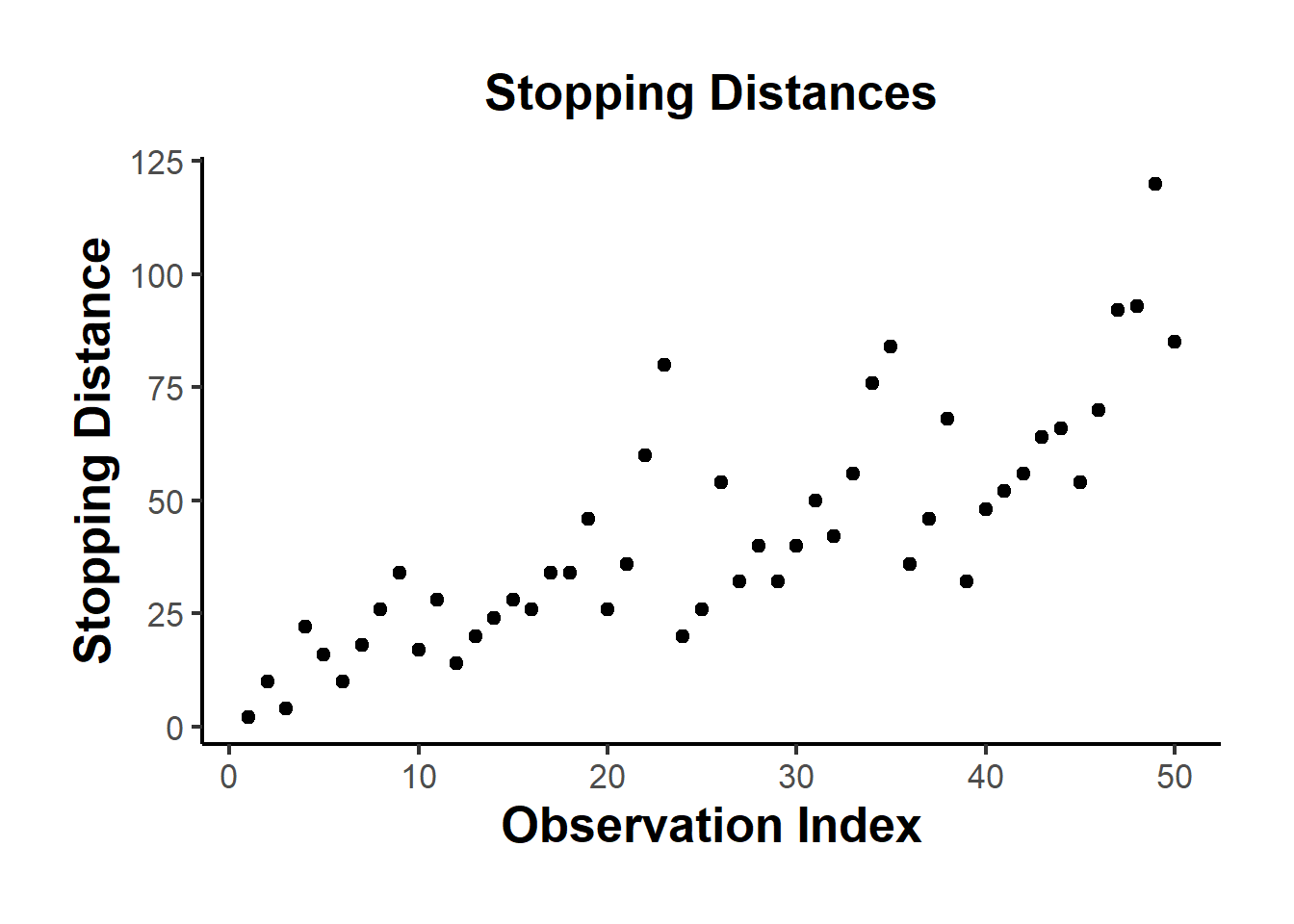
Figure 12.1: Stopping Distances
# Reciprocal transformation
library(ggplot2)
ggplot(cars, aes(x = seq_along(dist), y = 1/dist)) +
  geom_point(size = 2) +
  labs(
    title = "Stopping Distances",
    x     = "Observation Index",
    y     = "Reciprocal Stopping Distance"
  ) +
  theme_minimal(base_size = 14)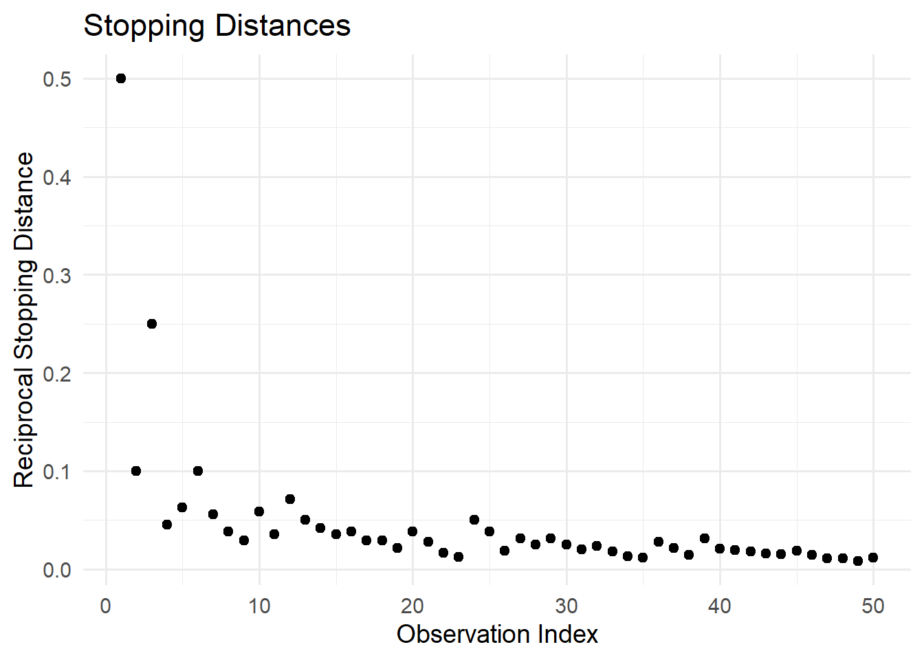
Figure 12.2: Reciprocal Stopping Distances
12.1.8 Hyperbolic Arcsine Transformation
The arcsinh (inverse hyperbolic sine) transformation is useful for handling proportion variables (0-1) and skewed distributions. It behaves similarly to the logarithmic transformation but has the advantage of handling zero and negative values.
Formula:
\[ \text{arcsinh}(Y) = \log(\sqrt{1 + Y^2} + Y) \]
When to Use:
Proportion variables (e.g., market share, probability estimates).
Data with extreme skewness where log transformation is problematic.
Variables containing zeros or negative values (unlike log, arcsinh handles zeros naturally).
Alternative to log transformation for handling zeros.
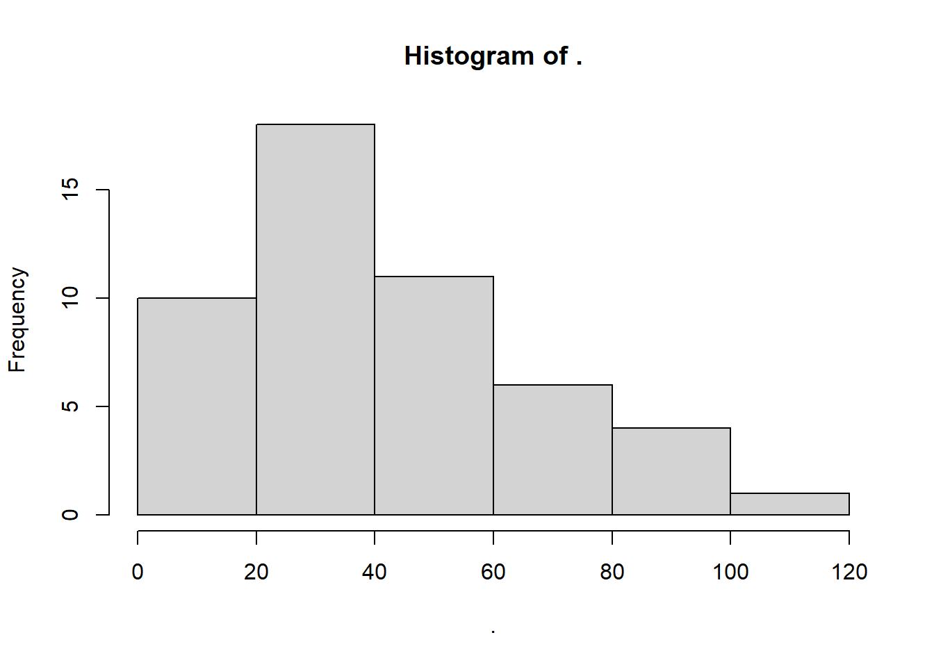
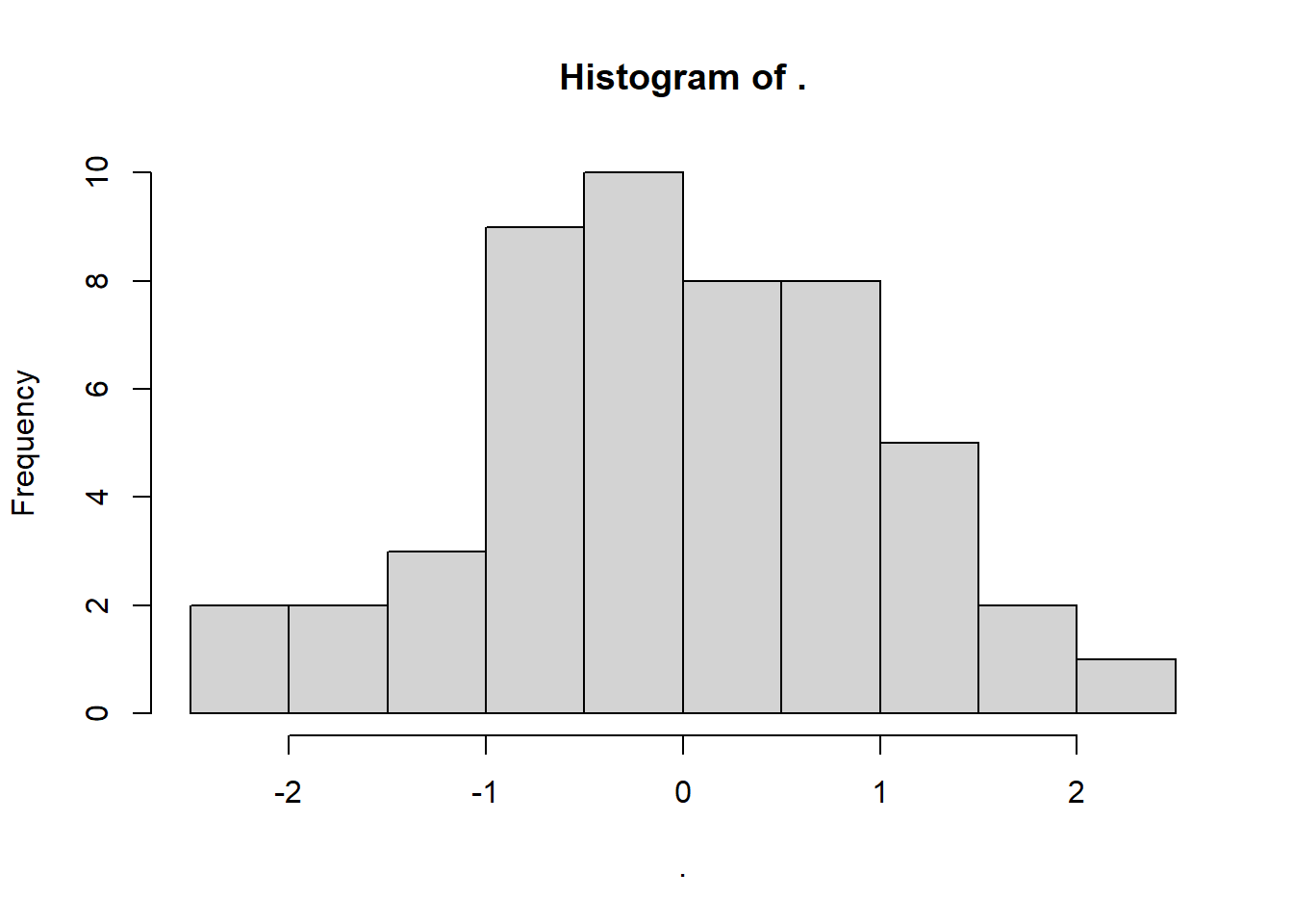
Figure 12.3: Histogram plot
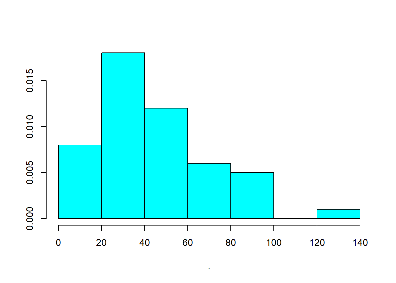
Figure 12.4: Alternative Histogram Plot
# Apply arcsinh transformation
as_dist <- bestNormalize::arcsinh_x(cars$dist)
as_dist
#> Standardized asinh(x) Transformation with 50 nonmissing obs.:
#>  Relevant statistics:
#>  - mean (before standardization) = 4.230843
#> - sd (before standardization) = 0.7710887library(ggplot2)
ggplot() +
geom_histogram(
aes(x = as_dist$x.t, y = after_stat(count)),
breaks = hist(as_dist$x.t, plot = FALSE)$breaks,
colour = "black",
fill = "lightblue"
) +
labs(
title = "Histogram of xt",
x = "xt values",
y = "Count"
) +
theme_minimal()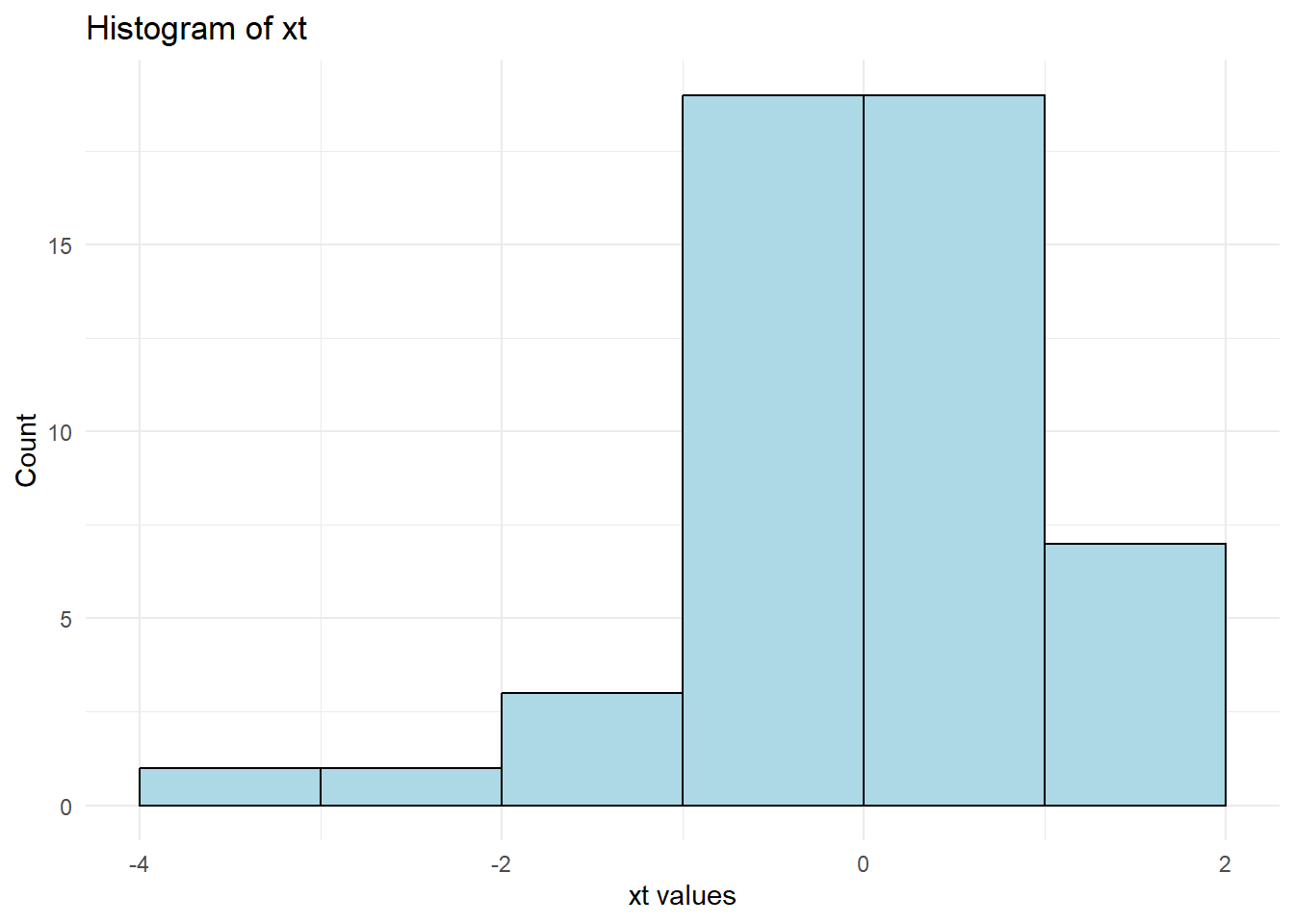
Figure 12.5: Arcsinh Transformed Histogram
| Paper | Interpretation |
|---|---|
| Azoulay, Fons-Rosen, and Zivin (2019) | Elasticity |
| Faber and Gaubert (2019) | Percentage |
| Hjort and Poulsen (2019) | Percentage |
| M. S. Johnson (2020) | Percentage |
| Beerli et al. (2021) | Percentage |
| Norris, Pecenco, and Weaver (2021) | Percentage |
| Berkouwer and Dean (2022) | Percentage |
| Cabral, Cui, and Dworsky (2022) | Elasticity |
| Carranza et al. (2022) | Percentage |
| Mirenda, Mocetti, and Rizzica (2022) | Percentage |
Consider a simple regression model: \[ Y = \beta X + \epsilon \] When both \(Y\) and \(X\) are transformed:
- The coefficient estimate \(\beta\) represents elasticity: A 1% increase in \(X\) leads to a \(\beta\)% change in \(Y\).
When only \(Y\) is transformed:
- The coefficient estimate represents a percentage change in \(Y\) for a one-unit change in \(X\).
This makes the arcsinh transformation particularly valuable for log-linear models where zero values exist.
12.1.9 Ordered Quantile Normalization (Rank-Based Transformation)
The Ordered Quantile Normalization (OQN) technique transforms data into a normal distribution using rank-based methods (Bartlett 1947).
Formula:
\[ x_i' = \Phi^{-1} \left( \frac{\text{rank}(x_i) - 1/2}{\text{length}(x)} \right) \]
where \(\Phi^{-1}\) is the inverse normal cumulative distribution function.
When to Use:
When data are heavily skewed or contain extreme values.
When normality is required for parametric tests.
ord_dist <- bestNormalize::orderNorm(cars$dist)
ord_dist
#> orderNorm Transformation with 50 nonmissing obs and ties
#>  - 35 unique values
#>  - Original quantiles:
#>   0%  25%  50%  75% 100%
#> 2 26 36 56 120library(ggplot2)
ggplot() +
geom_histogram(
aes(x = ord_dist$x.t, y = after_stat(count)),
breaks = hist(ord_dist$x.t, plot = FALSE)$breaks,
colour = "black",
fill = "lightblue"
) +
labs(
title = "Histogram",
x = "xt values",
y = "Count"
) +
theme_minimal()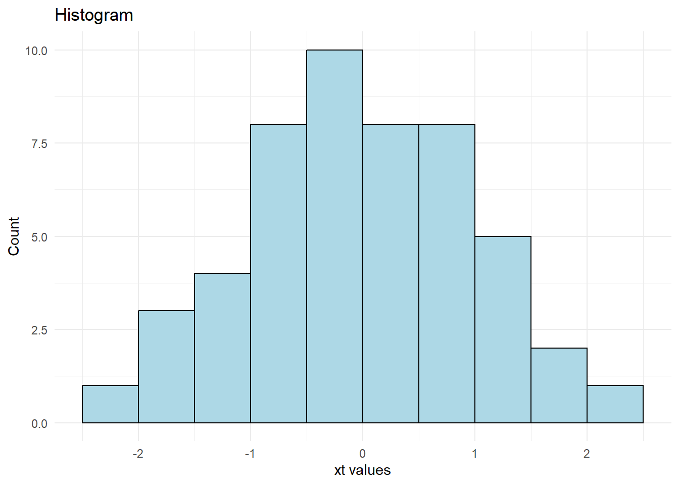
Figure 12.6: Histogram Plot
12.1.10 Lambert W x F Transformation
The Lambert W transformation is a more advanced method that normalizes data by removing skewness and heavy tails.
When to Use:
When traditional transformations (e.g., log, Box-Cox) fail.
When dealing with heavy-tailed distributions.
# cars = datasets::cars
# head(cars$dist)
# cars$dist %>% hist()

# Apply Lambert W transformation
l_dist <- LambertW::Gaussianize(cars$dist)library(ggplot2)
ggplot() +
geom_histogram(
aes(x = l_dist, y = after_stat(count)),
breaks = hist(l_dist, plot = FALSE)$breaks,
colour = "black",
fill = "lightblue"
) +
labs(
title = "Histogram of l_dist",
x = "l_dist values",
y = "Count"
) +
theme_minimal()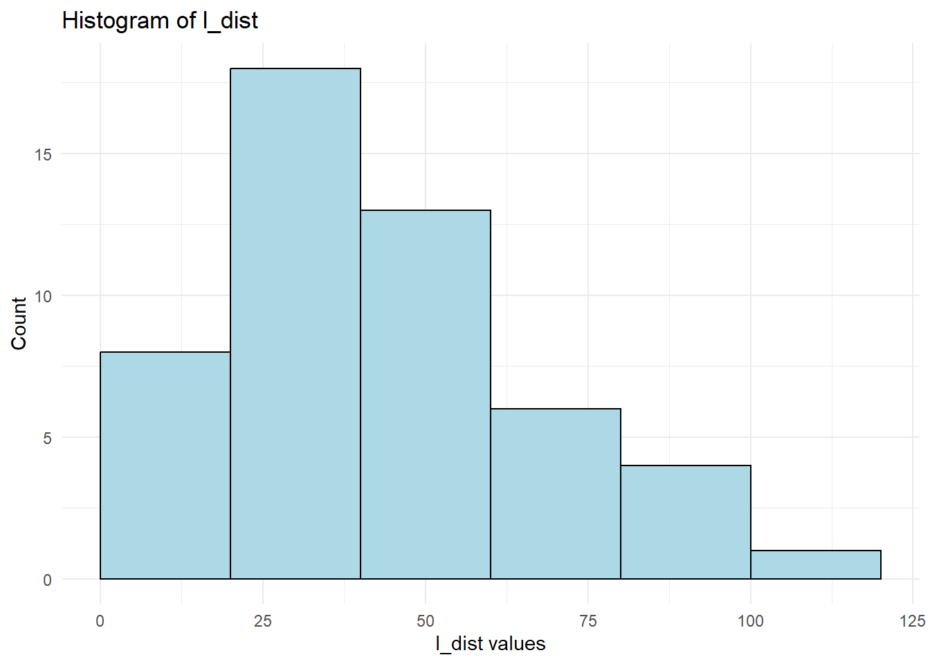
Figure 12.7: Lambert W Transformation
12.1.11 Inverse Hyperbolic Sine Transformation
The Inverse Hyperbolic Sine (IHS) transformation is similar to the log transformation but handles zero and negative values (N. L. Johnson 1949).
Formula:
\[ f(x,\theta) = \frac{\sinh^{-1} (\theta x)}{\theta} = \frac{\log(\theta x + (\theta^2 x^2 + 1)^{1/2})}{\theta} \]
When to Use:
When data contain zeros or negative values.
Alternative to log transformation in economic and financial modeling.
12.1.12 Box-Cox Transformation
The Box-Cox transformation is a power transformation designed to improve linearity and normality (Manly 1976; Bickel and Doksum 1981; Box and Cox 1981).
Formula:
\[ x_i'^\lambda = \begin{cases} \frac{x_i^\lambda-1}{\lambda} & \text{if } \lambda \neq 0\\ \log(x_i) & \text{if } \lambda = 0 \end{cases} \]
When to Use:
To fix non-linearity in the error terms of regression models.
When data are strictly positive
library(MASS)
# data(cars)
cars = datasets::cars
mod <- lm(cars$speed ~ cars$dist, data = cars)

# Check residuals
# plot(mod)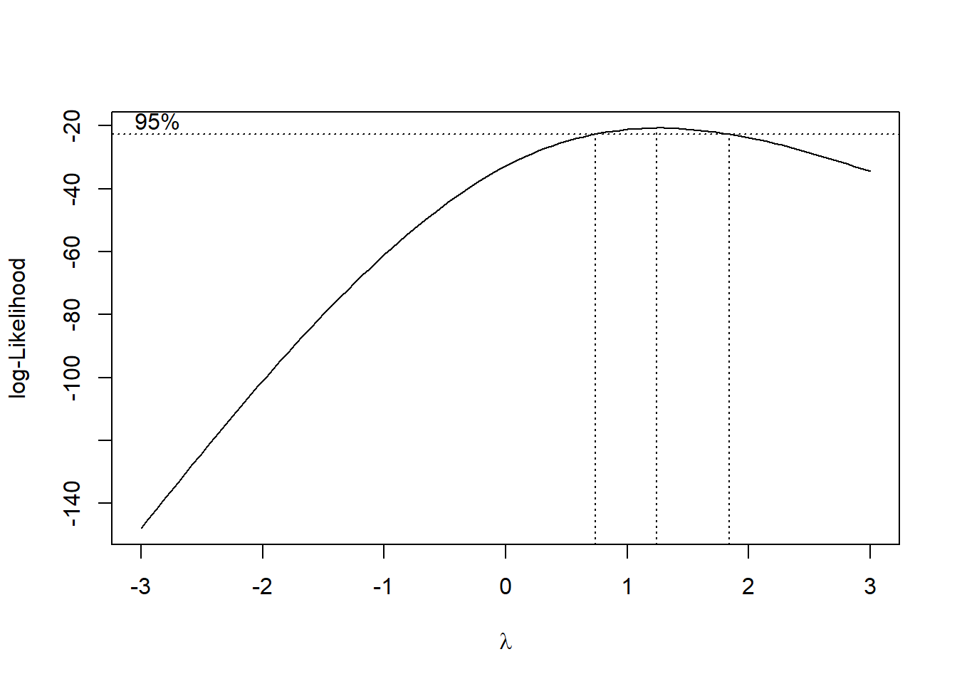
Figure 12.8: Log-likelihood Curve
best_lambda <- bc$x[which.max(bc$y)]

# Apply transformation
mod_lambda = lm(cars$speed ^ best_lambda ~ cars$dist, data = cars)
# plot(mod_lambda)
For the two-parameter Box-Cox transformation, we use:
\[ x_i' (\lambda_1, \lambda_2) = \begin{cases} \frac{(x_i + \lambda_2)^{\lambda_1}-1}{\lambda_1} & \text{if } \lambda_1 \neq 0 \\ \log(x_i + \lambda_2) & \text{if } \lambda_1 = 0 \end{cases} \]
12.1.13 Yeo-Johnson Transformation
Similar to Box-Cox (when \(\lambda = 1\)), but allows for negative values.
Formula:
\[ x_i'^\lambda = \begin{cases} \frac{(x_i+1)^\lambda -1}{\lambda} & \text{if } \lambda \neq0, x_i \ge 0 \\ \log(x_i + 1) & \text{if } \lambda = 0, x_i \ge 0 \\ \frac{-[(-x_i+1)^{2-\lambda}-1]}{2 - \lambda} & \text{if } \lambda \neq 2, x_i <0 \\ -\log(-x_i + 1) & \text{if } \lambda = 2, x_i <0 \end{cases} \]
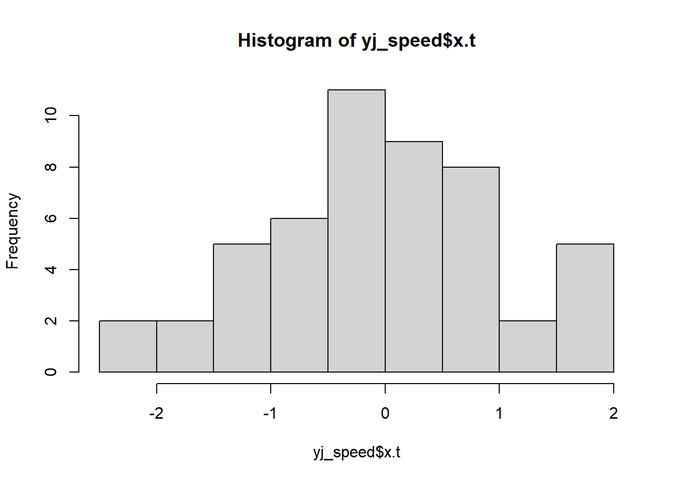
Figure 12.9: Histogram of xt