42.3 Coefficient Stability
Beyond specification curve analysis, another crucial aspect of sensitivity analysis is assessing whether your estimates are robust to potential omitted variable bias (Altonji, Elder, and Taber 2005). Even with comprehensive controls, unobserved confounders may threaten causal inference.
42.3.1 Theoretical Foundation: The Oster (2019) Approach
Oster’s (2019) influential paper provides a formal framework for assessing omitted variable bias. The key insight is that coefficient stability alone is insufficient, we need to consider both coefficient stability and \(R^2\) movement to evaluate the likely impact of unobservables.
The intuition is as follows:
- Coefficient stability: How much does the coefficient on your treatment variable change when you add controls?
- \(R^2\) movement: How much does the model’s explanatory power increase when you add controls?
If adding observed controls moves the \(R^2\) substantially but barely affects the coefficient, this suggests that unobservables (which might also affect \(R^2\)) are unlikely to overturn your result. Conversely, if the coefficient is very sensitive to the controls you add, unobservables might also have large effects.
Oster formalizes this by computing a parameter \(\delta\) (delta), which represents how strong the relationship between unobservables and the outcome would need to be (relative to the observables) to explain away the entire treatment effect. Higher values of \(\delta\) suggest more robust results.
The formula for calculating the bias-adjusted treatment effect is:
\[ \beta^* = \tilde{\beta} - \delta \times [\dot{\beta} - \tilde{\beta}] \times \frac{R_{max} - \tilde{R}^2}{\tilde{R}^2 - \dot{R}^2} \]
Where:
- \(\beta^*\) = bias-adjusted treatment effect
- \(\dot{\beta}\) = coefficient from short regression (without controls)
- \(\tilde{\beta}\) = coefficient from full regression (with controls)
- \(\dot{R}^2\) = \(R^2\) from short regression
- \(\tilde{R}^2\) = \(R^2\) from full regression
- \(R_{max}\) = hypothetical maximum \(R^2\) (often set to 1 or a realistic upper bound)
- \(\delta\) = proportional selection on unobservables (assumed relationship)
42.3.2 The robomit Package
The robomit package provides a straightforward implementation of Oster’s method:
library(robomit)

# Calculate bias-adjusted treatment effect using Oster's method
# This function estimates beta* under different assumptions about delta

o_beta_results = o_beta(
  y     = "mpg",        # Dependent variable
  x     = "wt",         # Treatment variable of interest
  con   = "hp + qsec",  # Control variables (covariates)
  delta = 1,            # Proportional selection assumption
                        # delta = 1 means unobservables are as important as observables
                        # delta = 0 means no omitted variable bias
                        # delta > 1 means unobservables are more important than observables
  R2max = 0.9,          # Maximum R-squared achievable
                        # Common choices: 1.0 (theoretical max),
                        # 1.3*R2_full (30% improvement over full model),
                        # or domain-specific reasonable maximum
  type  = "lm",         # Model type: "lm" for OLS, "logit" for logistic
  data  = mtcars        # Dataset
)
The function returns:
Coefficient from short model (without controls)
Coefficient from full model (with controls)
Bias-adjusted coefficient under delta and \(R^2\) max assumptions
The value of delta needed to drive the coefficient to zero
print(o_beta_results)
#> # A tibble: 10 × 2
#>    Name                           Value
#>    <chr>                          <dbl>
#>  1 beta*                         -2.00
#>  2 (beta*-beta controlled)^2      5.56
#>  3 Alternative Solution 1        -7.01
#>  4 (beta[AS1]-beta controlled)^2  7.05
#>  5 Uncontrolled Coefficient      -5.34
#>  6 Controlled Coefficient        -4.36
#>  7 Uncontrolled R-square          0.753
#>  8 Controlled R-square            0.835
#>  9 Max R-square                   0.9
#> 10 delta                          1
Interpretation:
If bias-adjusted beta is still large and significant, this suggests robustness to omitted variable bias
If the delta needed to explain away the effect is large (>1), this suggests you’d need very strong unobservables to overturn the result
For a more comprehensive analysis, you can explore coefficient stability across a range of delta values:
# Create a sequence of delta values to explore
delta_values = seq(0, 2, by = 0.1)

beta_results = sapply(delta_values, function(d) {
  result = suppressWarnings(
    o_beta(
      y = "mpg",
      x = "wt",
      con = "hp + qsec",
      delta = d,
      R2max = 0.9,
      type = "lm",
      data = mtcars
    )
  )
  # Extract beta* (first row)
  result$Value[result$Name == "beta*"]
})

# Create visualization
stability_df = data.frame(
  delta = delta_values,
  beta_adjusted = beta_results
)
Interpretation guidelines:
\(|\delta| < 1\): Unobservables would need to be less related to treatment/outcome than observables to overturn the result (less robust)
\(|\delta| \approx 1\): Unobservables would need to be about as related as observables (moderate robustness)
\(|\delta| > 1\): Unobservables would need to be MORE related than observables (more robust)
\(|\delta| >> 1\): Very robust to omitted variable bias
Figure 42.8 shows bias-adjusted coefficients against \(\delta\)
# Plot
library(ggplot2)
ggplot(stability_df, aes(x = delta, y = beta_adjusted)) +
  geom_line(linewidth = 1) +
  geom_hline(yintercept = 0, linetype = "dashed", color = "red") +
  labs(
    x = "Delta (strength of confounding)",
    y = "Bias-adjusted coefficient (beta*)",
    title = "Coefficient stability under omitted variable bias"
  ) +
  theme_minimal()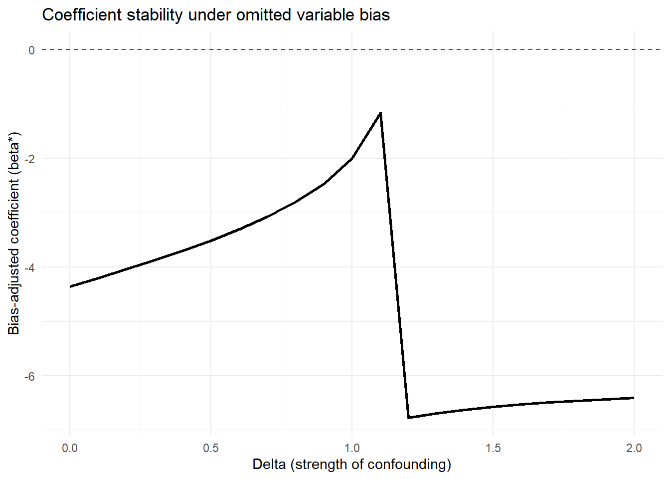
Figure 42.8: Coefficient stability under omitted variable bias
For more sophisticated applications with multiple treatments or different model types:
# Example with multiple treatment variables
# Useful when you have several key independent variables of interest

results_multi = lapply(c("wt", "hp"), function(treat) {
  o_beta(
    y = "mpg",
    x = treat,
    con = "qsec + gear + carb",  # More extensive controls
    delta = 1,
    R2max = 1.0,  # Theoretical maximum
    type = "lm",
    data = mtcars
  )
})

names(results_multi) = c("wt", "hp")
print(results_multi)
#> $wt
#> # A tibble: 10 × 2
#>    Name                           Value
#>    <chr>                          <dbl>
#>  1 beta*                          4.56
#>  2 (beta*-beta controlled)^2     68.3
#>  3 Alternative Solution 1        -6.29
#>  4 (beta[AS1]-beta controlled)^2  6.70
#>  5 Uncontrolled Coefficient      -5.34
#>  6 Controlled Coefficient        -3.70
#>  7 Uncontrolled R-square          0.753
#>  8 Controlled R-square            0.845
#>  9 Max R-square                   1
#> 10 delta                          1
#>
#> $hp
#> # A tibble: 10 × 2
#>    Name                             Value
#>    <chr>                            <dbl>
#>  1 beta*                          0.118
#>  2 (beta*-beta controlled)^2      0.0250
#>  3 Alternative Solution 1        -0.0848
#>  4 (beta[AS1]-beta controlled)^2  0.00195
#>  5 Uncontrolled Coefficient      -0.0682
#>  6 Controlled Coefficient        -0.0406
#>  7 Uncontrolled R-square          0.602
#>  8 Controlled R-square            0.794
#>  9 Max R-square                   1
#> 10 delta                          1
Comparing robustness across treatment variables helps identify which relationships are most stable.
42.3.3 The mplot Package for Graphical Model Stability
The mplot package provides complementary tools for visualizing model stability and variable selection:
# Install if needed
# install.packages("mplot")
library(mplot)

# Visualize variable importance across models
mplot::vis(
  lm(mpg ~ wt + hp + qsec + gear + carb, data = mtcars),
  B = 100  # Number of bootstrap samples
)
#>                      name prob logLikelihood
#>                     mpg~1 1.00       -102.38
#>                    mpg~wt 0.97        -80.01
#>                 mpg~wt+hp 0.45        -74.33
#>               mpg~wt+qsec 0.36        -74.36
#>  mpg~wt+qsec+gear+carb+RV 0.39        -71.46
This creates plots showing:
- Which variables are selected across bootstrap samples
- Coefficient stability for each variable
- Model fit across different variable combinations
Particularly useful for:
Assessing variable importance
Understanding multicollinearity effects
Evaluating model selection stability