42.5 Advanced Topics in Sensitivity Analysis

42.5.1 Sensitivity to Outliers and Influential Observations

Outliers can drive results, so it’s important to assess robustness to their inclusion:

# Identify influential observations
model = lm(mpg ~ wt + hp + qsec, data = mtcars)

# Calculate influence measures
influence_measures = influence.measures(model)

# Cook's Distance
cooks_d = cooks.distance(model)
influential = cooks_d > 4 / nrow(mtcars)  # Common threshold

# DFBETAS (change in coefficient when observation removed)
dfbetas_vals = dfbetas(model)

# Compare models with/without influential observations
model_full = lm(mpg ~ wt + hp + qsec, data = mtcars)
model_no_influential = lm(
  mpg ~ wt + hp + qsec,
  data = mtcars[!influential, ]
)

# Compare coefficients
compare_df = data.frame(
  Variable = names(coef(model_full)),
  Full_Sample = coef(model_full),
  Excl_Influential = c(
    coef(model_no_influential),
    rep(NA, length(coef(model_full)) - length(coef(model_no_influential)))
  )
)

# Winsorization approach
library(DescTools)
mtcars_winsor = mtcars
mtcars_winsor$wt = DescTools::Winsorize(mtcars$wt, val = c(0.01, 0.99))
mtcars_winsor$hp = DescTools::Winsorize(mtcars$hp, val = c(0.01, 0.99))

model_winsor = lm(mpg ~ wt + hp + qsec, data = mtcars_winsor)

# Compare original vs. winsorized

42.5.2 Sensitivity to Measurement Error

If key variables are measured with error, results may be biased:

# Simulate measurement error
# This helps understand potential attenuation bias

library(simex)

# SIMEX (Simulation-Extrapolation) for measurement error correction
# Assumes classical measurement error in covariates

# Fit model with x = TRUE
naive_model <- lm(mpg ~ wt + hp, data = mtcars, x = TRUE)

# Apply SIMEX
# lambda is the factor by which measurement error variance increases
simex_model <- simex(
  naive_model,
  SIMEXvariable = "wt",  # Variable with measurement error
  measurement.error = 0.1,  # Assumed ME variance (proportion of var)
  lambda = seq(0.1, 2, 0.1),  # Extrapolation sequence
  B = 100  # Number of simulations
)


# View results
summary(simex_model)
#> Call:
#> simex(model = naive_model, SIMEXvariable = "wt", measurement.error = 0.1, 
#>     lambda = seq(0.1, 2, 0.1), B = 100)
#> 
#> Naive model: 
#> lm(formula = mpg ~ wt + hp, data = mtcars, x = TRUE)
#> 
#> Simex variable :
#>                      wt
#> Measurement error : 0.1
#> 
#> 
#> Number of iterations:  100 
#> 
#> Residuals: 
#>      Min.   1st Qu.    Median      Mean   3rd Qu.      Max. 
#> -3.931701 -1.603200 -0.225173 -0.007991  1.066691  5.806683 
#> 
#> Coefficients: 
#> 
#> Asymptotic variance: 
#>              Estimate Std. Error t value Pr(>|t|)    
#> (Intercept) 37.376807   1.987465  18.806  < 2e-16 ***
#> wt          -3.974826   0.644667  -6.166 1.01e-06 ***
#> hp          -0.030611   0.006577  -4.654 6.63e-05 ***
#> ---
#> Signif. codes:  0 '***' 0.001 '**' 0.01 '*' 0.05 '.' 0.1 ' ' 1
#> 
#> Jackknife variance: 
#>              Estimate Std. Error t value Pr(>|t|)    
#> (Intercept) 37.376807   1.583219  23.608  < 2e-16 ***
#> wt          -3.974826   0.636895  -6.241 8.24e-07 ***
#> hp          -0.030611   0.009077  -3.372  0.00213 ** 
#> ---
#> Signif. codes:  0 '***' 0.001 '**' 0.01 '*' 0.05 '.' 0.1 ' ' 1

# Compare naive vs corrected coefficients
data.frame(
  Coefficient = names(coef(naive_model)),
  Naive = coef(naive_model),
  SIMEX_Corrected = coef(simex_model)
)
#>             Coefficient       Naive SIMEX_Corrected
#> (Intercept) (Intercept) 37.22727012     37.37680699
#> wt                   wt -3.87783074     -3.97482594
#> hp                   hp -0.03177295     -0.03061053

# SIMEX extrapolates back to zero ME, giving corrected estimate

Figure 42.11 plots SIMEX extrapolation.

# Plot SIMEX extrapolation
par(mfrow = c(1, 3))
plot(simex_model)

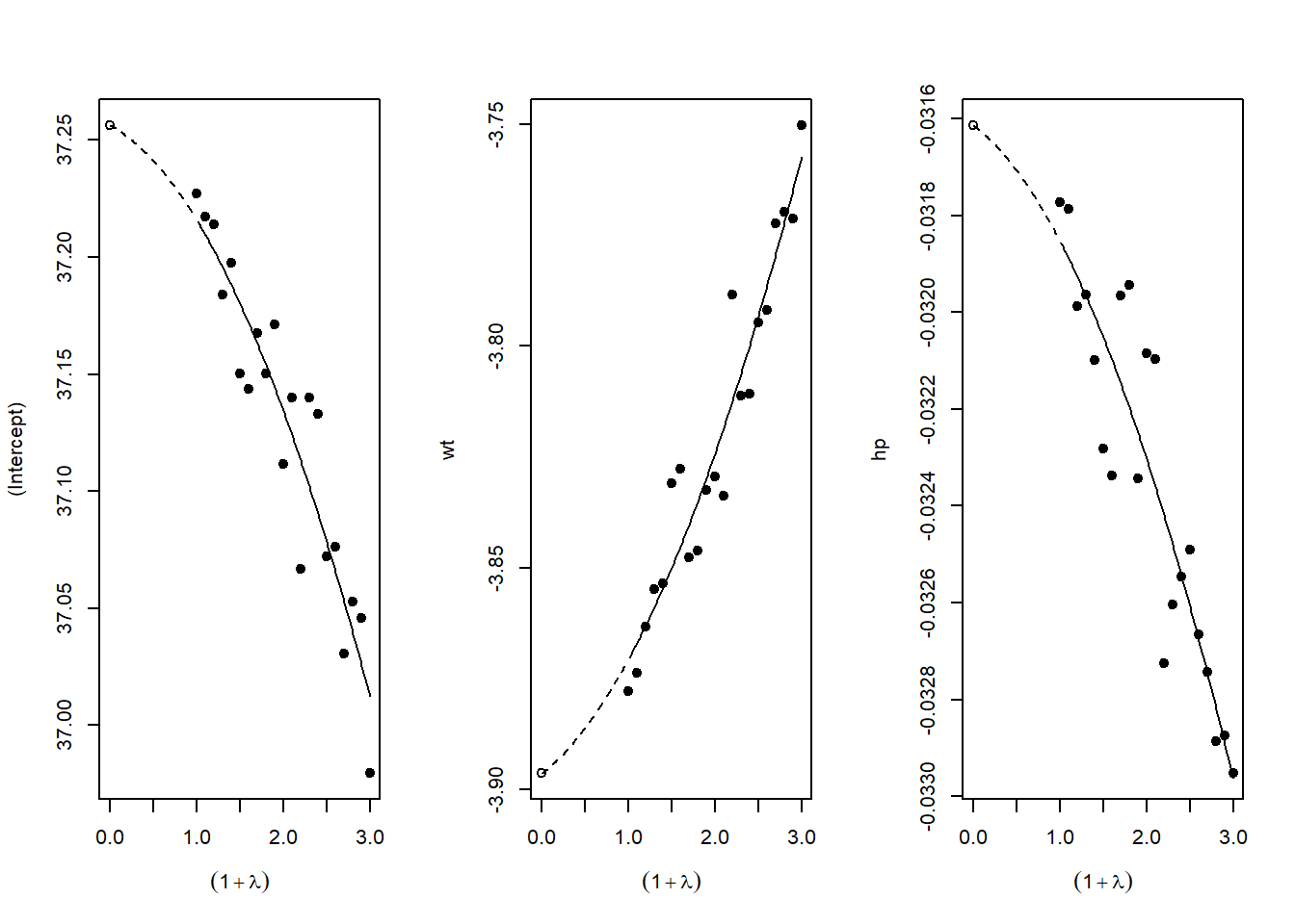
Figure 42.11: SIMEX extrapolation plots for measurement error correction

par(mfrow = c(1, 1))

---